R システムのパッケージに付属のデータセットから SQLite 3 データベースを生成（R システム，SQLite3 を使用）

次のデータから SQLite 3 データベースを生成する．

一般: iris, diamonds, Indometh
時系列: Lai2005fig4, meteoandes, economics , nhtemp
緯度・経度: seals

◆ 作成するSQLite 3 データベース:rdataset

前準備

使用するソフトウェア

R システムのインストールが済んでいること
SQLite 3 のインストール: SQLite 3インストール，データベース作成，テーブル定義，レコード挿入（Windows 上）別ページ »で説明
python のインストール、python のパッケージ sqlite3, rpy2, numpy, pandas のインストールが済んでいること

あらかじめ決めておく事項

このページでは，SQLite 3 データベースの生成を行う．生成するSQLite 3 データベースのデータベース名を決めておくこと．このページでは，次のように書く．

データベース名: rdataset
データベース名は，自由に決めてよいが，半角文字（つまり英字と英記号）を使い，スペースを含まないこと，

一般のデータ

iris

テーブル定義

iris(Sepal_Length, Sepal_Width, Petal_Length, Petal_Width, Species)

◆ bash プログラム

#!/usr/bin/python

import sqlite3
conn = sqlite3.connect('rdataset')

sql = u"""
drop table iris; 
"""
conn.execute(sql)

sql = u"""
create table iris ( 
  Sepal_Length  real, 
  Sepal_Width   real,
  Petal_Length  real,
  Petal_Width   real, 
  Species       text 
);  
"""
conn.execute(sql)

conn.close()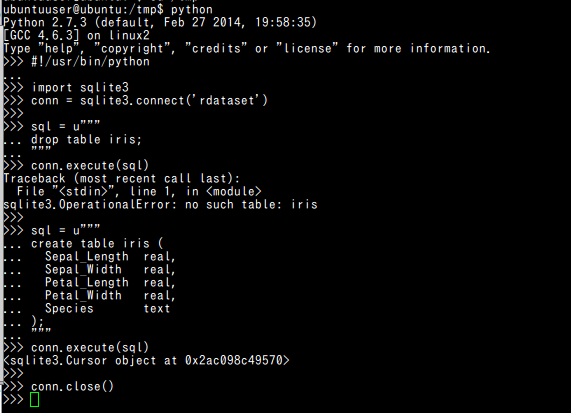

テーブルの作成

◆ bash プログラム

#!/usr/bin/python

import rpy2.robjects
import pandas.rpy.common

x = pandas.rpy.common.load_data('iris') 
for i in x:
  print '==='
  print i


cat /tmp/a.$$.r | R --no-save

cat >/tmp/a.$$.sql <<-SQL
.mode csv
.import /tmp/a.$$.csv iris
vacuum; 
SQL
#
tail -n +2 /tmp/iris.csv > /tmp/a.$$.csv
cat /tmp/a.$$.sql | sqlite3 /tmp/rdataset
# 
echo 'select * from iris limit 10;' | sqlite3 /tmp/rdataset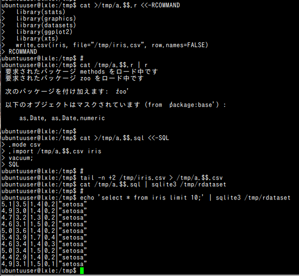

diamonds

テーブル定義

diamonds(carat, cut, color, clarity, depth, table, price, x, y, z)

◆ bash プログラム

#!/bin/bash

# rm -f /tmp/rdataset
#
cat >/tmp/a.$$.sql <<-SQL
drop table diamonds; 
SQL
cat /tmp/a.$$.sql | sqlite3 /tmp/rdataset
#
cat >/tmp/a.$$.sql <<-SQL
create table diamonds (
  carat   real,
  cut     text, 
  color   text, 
  clarity text, 
  depth   real, 
  tbl     real, 
  price   integer, 
  x       real, 
  y       real, 
  z       real
);  
SQL
cat /tmp/a.$$.sql | sqlite3 /tmp/rdataset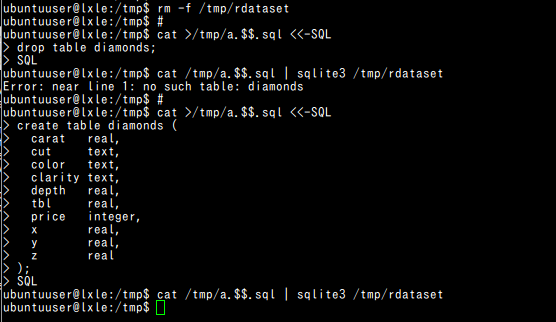

テーブルの作成

◆ bash プログラム

#!/bin/bash

cat >/tmp/a.$$.r <<-RCOMMAND
  library(stats)
  library(graphics)
  library(datasets)
  library(ggplot2)
  library(xts)
  library(chron)
  write.csv(diamonds, file="/tmp/diamonds.csv", row.names=FALSE)
RCOMMAND
#
cat /tmp/a.$$.r | R --no-save

cat >/tmp/a.$$.sql <<-SQL
.mode csv
.import /tmp/a.$$.csv diamonds
vacuum; 
SQL
#
tail -n +2 /tmp/diamonds.csv > /tmp/a.$$.csv
cat /tmp/a.$$.sql | sqlite3 /tmp/rdataset
# 
echo 'select * from diamonds limit 10;' | sqlite3 /tmp/rdataset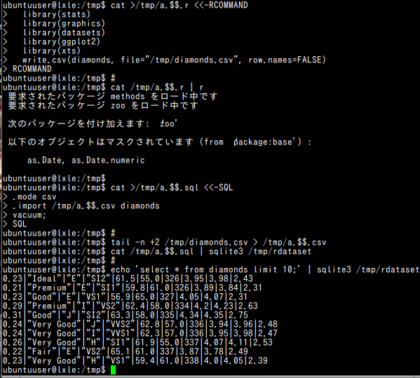

Indometh

テーブル定義

Indometh(Subject, t, conc)

◆ bash プログラム

#!/bin/bash

# rm -f /tmp/rdataset
#
cat >/tmp/a.$$.sql <<-SQL
drop table Indometh; 
SQL
cat /tmp/a.$$.sql | sqlite3 /tmp/rdataset
#
cat >/tmp/a.$$.sql <<-SQL
create table Indometh (
  Subject  integer, 
  t        real, 
  conc     real
);  
SQL
cat /tmp/a.$$.sql | sqlite3 /tmp/rdataset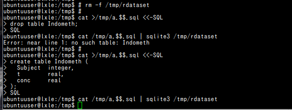

テーブルの作成

◆ bash プログラム

#!/bin/bash

cat >/tmp/a.$$.r <<-RCOMMAND
  library(stats)
  library(graphics)
  library(datasets)
  library(ggplot2)
  library(xts)
  library(chron)
  write.csv(Indometh, file="/tmp/Indometh.csv", row.names=FALSE)
RCOMMAND
#
cat /tmp/a.$$.r | R --no-save

cat >/tmp/a.$$.sql <<-SQL
.mode csv
.import /tmp/a.$$.csv Indometh
vacuum; 
SQL
#
tail -n +2 /tmp/Indometh.csv > /tmp/a.$$.csv
cat /tmp/a.$$.sql | sqlite3 /tmp/rdataset
# 
echo 'select * from Indometh limit 10;' | sqlite3 /tmp/rdataset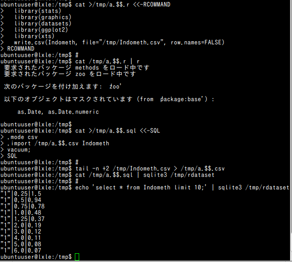

時系列 (time series)

wind

ここでの wind は gstat パッケージ内の風向データ

テーブル定義

wind(year, month, day, RPT, VAL, ROS, KIL, SHA, BIR, DUB, CLA, MUL, CLO, BEL, MAL)

◆ bash プログラム

#!/bin/bash

# rm -f /tmp/rdataset
#
cat >/tmp/a.$$.sql <<-SQL
drop table wind; 
SQL
cat /tmp/a.$$.sql | sqlite3 /tmp/rdataset
#
cat >/tmp/a.$$.sql <<-SQL
create table wind (
  at     date, 
  year   integer, 
  month  integer, 
  day    integer, 
  RPT    real, 
  VAL    real, 
  ROS    real, 
  KIL    real, 
  SHA    real, 
  BIR    real, 
  DUB    real, 
  CLA    real, 
  MUL    real, 
  CLO    real, 
  BEL    real, 
  MAL    real
);  
SQL
cat /tmp/a.$$.sql | sqlite3 /tmp/rdataset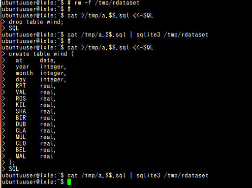

テーブルの作成

◆ bash プログラム

#!/bin/bash

cat >/tmp/a.$$.r <<-RCOMMAND
  library(stats)
  library(graphics)
  library(datasets)
  library(ggplot2)
  library(xts)
  library(chron)
  library(insol)
  library(gstat)
  data(wind)
  wind\$at = as.Date( ISOdate(wind\$year + 1900, wind\$month, wind\$day) )
  # 列順序の入れ替え
  wind <- wind[,c(16,1,2,3,4,5,6,7,8,9,10,11,12,13,14,15)]             
  str(wind)  
  write.csv(wind, file="/tmp/wind.csv", row.names=FALSE)
RCOMMAND
#
cat /tmp/a.$$.r | R --no-save

cat >/tmp/a.$$.sql <<-SQL
.mode csv
.import /tmp/a.$$.csv wind
vacuum; 
SQL
#
tail -n +2 /tmp/wind.csv > /tmp/a.$$.csv
cat /tmp/a.$$.sql | sqlite3 /tmp/rdataset
# 
echo 'select * from wind limit 10;' | sqlite3 /tmp/rdataset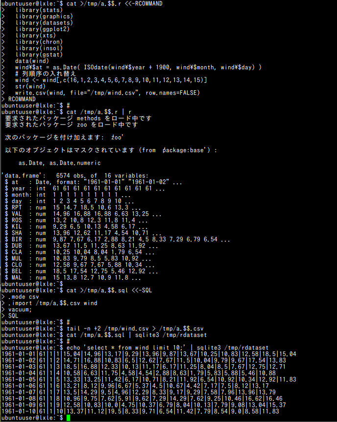

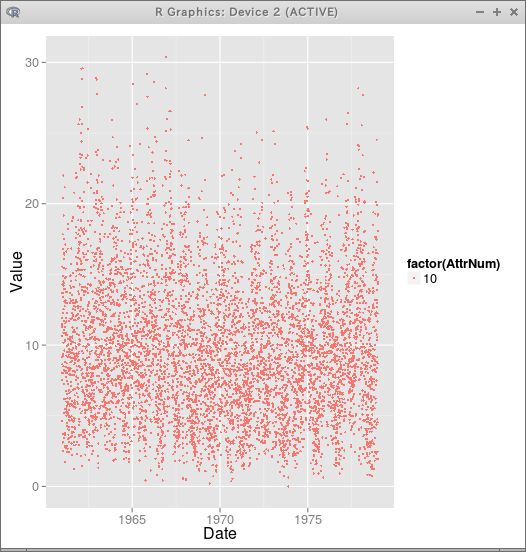
◆ ggplot() を使用 (R プログラム)　

  library(ggplot2)
  library(RSQLite)
  library(xts)
  library(chron)

  fetch_table <- function(sqlite3dbname, tablename) {
    drv <- dbDriver("SQLite", max.con = 1)
    conn <- dbConnect(drv, dbname=sqlite3dbname)
    rs <- dbSendQuery( conn, paste("SELECT * from", tablename, ";") )
    T <- fetch(rs, n = -1)
    return(T)
  }

  T <- fetch_table("/tmp/rdataset", "wind")

# 
  table_to_melt <- function(T, tsvec, tsformat) {
    # 先に xts 型に変換しておく
    D <- as.xts( read.zoo( T, tsformat ) )
    # melt(Date, AttrNum, Value). 
    Date <- rep(strptime(tsvec, tsformat, tz=""), ncol(D))
    AttrNum <- rep(1:ncol(D), each=nrow(D))
    Value <- as.numeric(as.vector(D))
    return( data.frame(Date=Date, AttrNum=AttrNum, Value=Value) )
  }
  
  M <- table_to_melt(T, T$at, "%Y-%m-%d")
#
#  ggplot(M, aes(x=Date, y=Value, colour=factor(AttrNum))) + geom_point(size=1);
  ggplot(subset(M, AttrNum==10), aes(x=Date, y=Value, colour=factor(AttrNum))) + geom_point(size=1);

◆ 追加プログラム (R プログラム)　（書きかけ）

http://www.inside-r.org/packages/cran/gstat/docs/wind

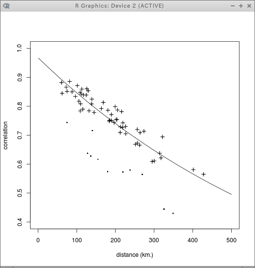
#  1月1日を基点とする日数（月日の情報を使う．年は無視）
j <- as.numeric(format(as.Date(T$at), '%j') ) 

winsqrt = sqrt( 0.5148 * ( as.matrix(T[5:16]) ) )
plot(winsqrt)
winsqrt = winsqrt - mean(winsqrt)
a <- sapply( split(winsqrt, j), mean )

plot(a)
lines( lowess(a, f=0.1) )

meteoandes

テーブル定義

meteoandes(year, doy, hh, mm, Tair, pyra1, pyra2, windspeed, winddir, RH)

◆ bash プログラム

#!/bin/bash

# rm -f /tmp/rdataset
#
cat >/tmp/a.$$.sql <<-SQL
drop table meteoandes; 
SQL
cat /tmp/a.$$.sql | sqlite3 /tmp/rdataset
#
cat >/tmp/a.$$.sql <<-SQL
create table meteoandes (
  meteodate datetime, 
  year      integer, 
  doy       integer, 
  hh        integer, 
  mm        integer, 
  Tair      real, 
  pyra1     real, 
  pyra2     real, 
  windspeed real, 
  winddir   real, 
  RH        real
);  
SQL
cat /tmp/a.$$.sql | sqlite3 /tmp/rdataset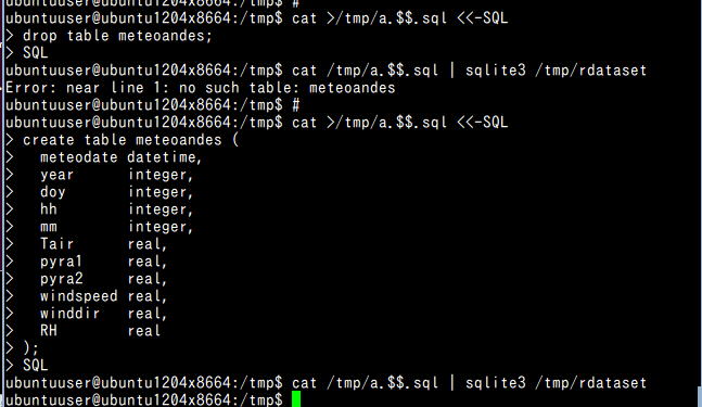

テーブルの作成

◆ bash プログラム

#!/bin/bash

cat >/tmp/a.$$.r <<-RCOMMAND
  library(stats)
  library(graphics)
  library(datasets)
  library(ggplot2)
  library(xts)
  library(chron)
  library(insol)
  data(meteoandes)
  meteoandes\$meteodate = strptime(paste(meteoandes\$year,meteoandes\$doy,meteoandes\$hh,meteoandes\$mm),format="%Y %j %H %M",tz="America/Santiago")
  # 列順序の入れ替え
  meteoandes <- meteoandes[,c(11,1,2,3,4,5,6,7,8,9,10)]             
  str(meteoandes)  
  write.csv(meteoandes, file="/tmp/meteoandes.csv", row.names=FALSE)
RCOMMAND
#
cat /tmp/a.$$.r | R --no-save

cat >/tmp/a.$$.sql <<-SQL
.mode csv
.import /tmp/a.$$.csv meteoandes
vacuum; 
SQL
#
tail -n +2 /tmp/meteoandes.csv > /tmp/a.$$.csv
cat /tmp/a.$$.sql | sqlite3 /tmp/rdataset
# 
echo 'select * from meteoandes limit 10;' | sqlite3 /tmp/rdataset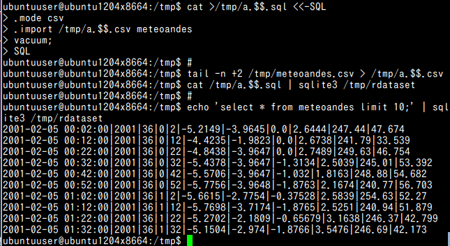

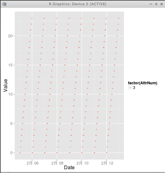
R のプログラム例を用いてプロット

◆ ggplot() を使用 (R プログラム)　(書きかけ)（動作未確認）

  library(ggplot2)
  library(RSQLite)
  library(xts)
  library(chron)

  fetch_table <- function(sqlite3dbname, tablename) {
    drv <- dbDriver("SQLite", max.con = 1)
    conn <- dbConnect(drv, dbname=sqlite3dbname)
    rs <- dbSendQuery( conn, paste("SELECT * from", tablename, ";") )
    T <- fetch(rs, n = -1)
    return(T)
  }

  T <- fetch_table("/tmp/rdataset", "meteoandes")

# 
  table_to_melt <- function(T, tsvec, tsformat) {
    # 先に xts 型に変換しておく
    D <- as.xts( read.zoo( T, tsformat ) )
    # melt(Date, AttrNum, Value). 
    Date <- rep(strptime(tsvec, tsformat, tz=""), ncol(D))
    AttrNum <- rep(1:ncol(D), each=nrow(D))
    Value <- as.numeric(as.vector(D))
    return( data.frame(Date=Date, AttrNum=AttrNum, Value=Value) )
  }
  
  M <- table_to_melt(T, T$meteodate, "%Y-%m-%d %H:%M:%S")
#
  ggplot(M, aes(x=Date, y=Value, colour=factor(AttrNum))) + geom_point(size=1);
#
  ggplot(subset(M, AttrNum==3), aes(x=Date, y=Value, colour=factor(AttrNum))) + geom_point(size=1);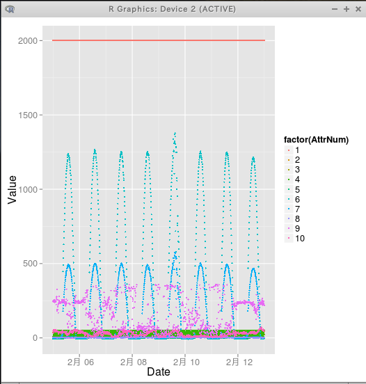

◆ plot() を使用 (R プログラム)

  library(RSQLite)
  library(xts)
  library(chron)
  drv <- dbDriver("SQLite", max.con = 1)
  conn <- dbConnect(drv, dbname="/tmp/rdataset")
  rs <- dbSendQuery( conn, "SELECT * from meteoandes;" )
  T <- fetch(rs, n = -1)
# plot pyra1, pyra2 
  plot(strptime(T$meteodate, "%Y-%m-%d %H:%M:%S", tz=""), T$pyra1, 'l', col=2, xlab='Date', xaxt="n",  
  ylab=expression(paste('Solar radiation [ ',Wm^-2,' ]')), main='Insolation at Loma Larga glacier')
  r <- as.POSIXct(round(range(strptime(T$meteodate, "%Y-%m-%d %H:%M:%S", tz="")), "days"))
  lines(strptime(T$meteodate, "%Y-%m-%d %H:%M:%S", tz=""), T$pyra2, col=4)
  axis.POSIXct(1, at=seq(r[1],r[2], by="1 week"), format="%d日　0時")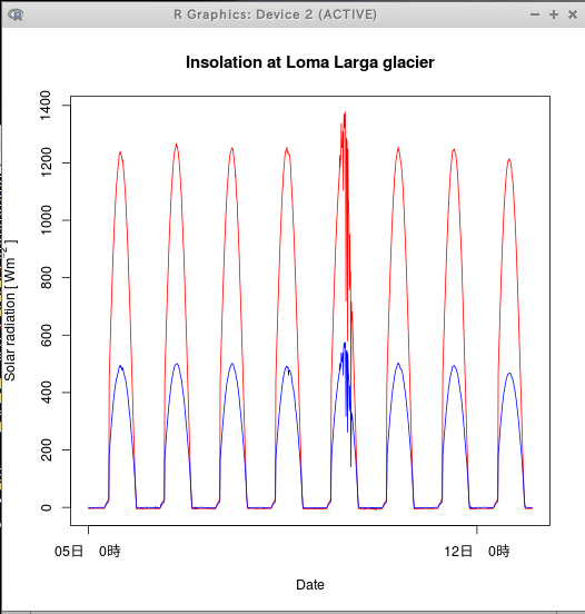

economics

テーブル定義

economics(dt, pce, pop, psavert, uempmed, unemploy)

◆ bash プログラム

#!/bin/bash

# rm -f /tmp/rdataset
#
cat >/tmp/a.$$.sql <<-SQL
drop table economics; 
SQL
cat /tmp/a.$$.sql | sqlite3 /tmp/rdataset
#
cat >/tmp/a.$$.sql <<-SQL
create table economics (
  dt       datetime, 
  pce      real, 
  pop      integer,
  psavert  real, 
  uempmed  real, 
  unemploy integer 
);  
SQL
cat /tmp/a.$$.sql | sqlite3 /tmp/rdataset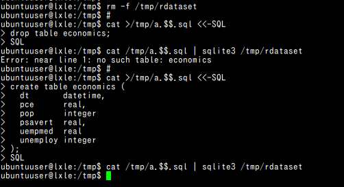

テーブルの作成

◆ bash プログラム

#!/bin/bash

cat >/tmp/a.$$.r <<-RCOMMAND
  library(stats)
  library(graphics)
  library(datasets)
  library(ggplot2)
  library(xts)
  library(chron)
  write.csv(economics, file="/tmp/economics.csv", row.names=FALSE)
RCOMMAND
#
cat /tmp/a.$$.r | R --no-save

cat >/tmp/a.$$.sql <<-SQL
.mode csv
.import /tmp/a.$$.csv economics
vacuum; 
SQL
#
tail -n +2 /tmp/economics.csv > /tmp/a.$$.csv
cat /tmp/a.$$.sql | sqlite3 /tmp/rdataset
# 
echo 'select * from economics limit 10;' | sqlite3 /tmp/rdataset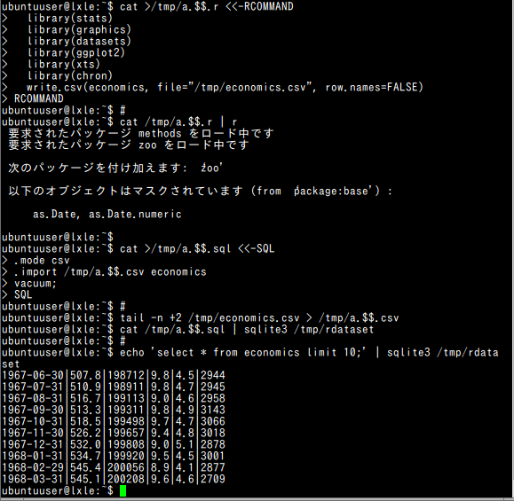

R のプログラム例を用いてプロット

◆ ggplot() を使用 (R プログラム)　

  library(ggplot2)
  library(RSQLite)
  library(xts)
  library(chron)

  fetch_table <- function(sqlite3dbname, tablename) {
    drv <- dbDriver("SQLite", max.con = 1)
    conn <- dbConnect(drv, dbname=sqlite3dbname)
    rs <- dbSendQuery( conn, paste("SELECT * from", tablename, ";") )
    T <- fetch(rs, n = -1)
    return(T)
  }

  T <- fetch_table("/tmp/rdataset", "economics")

# 
  table_to_melt <- function(T, tsvec, tsformat) {
    # 先に xts 型に変換しておく
    D <- as.xts( read.zoo( T, tsformat ) )
    # melt(Date, AttrNum, Value). 
    Date <- rep(strptime(tsvec, tsformat, tz=""), ncol(D))
    AttrNum <- rep(1:ncol(D), each=nrow(D))
    Value <- as.numeric(as.vector(D))
    return( data.frame(Date=Date, AttrNum=AttrNum, Value=Value) )
  }
  
  M <- table_to_melt(T, T$dt, "%Y-%m-%d")
#
  ggplot(M, aes(x=Date, y=Value, colour=factor(AttrNum))) + geom_point(size=1);
#
  ggplot(subset(M, AttrNum==3), aes(x=Date, y=Value, colour=factor(AttrNum))) + geom_point(size=1);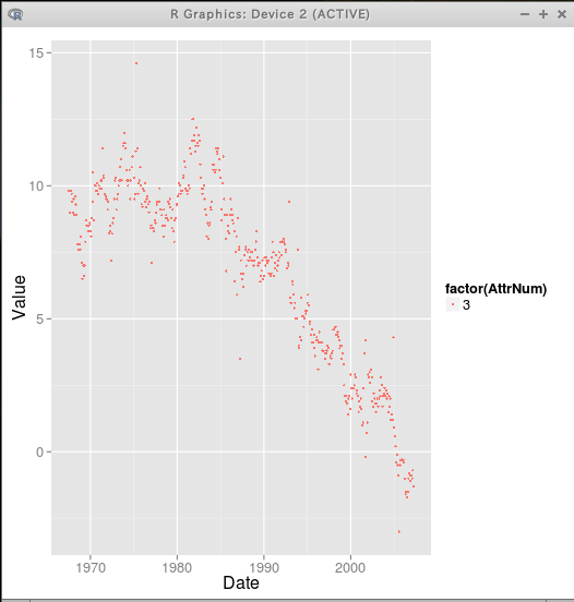

nhtemp

テーブル定義

nhtemp(ts, temperature)

◆ bash プログラム

#!/bin/bash

# rm -f /tmp/rdataset
#
cat >/tmp/a.$$.sql <<-SQL
drop table nhtemp; 
SQL
cat /tmp/a.$$.sql | sqlite3 /tmp/rdataset
#
cat >/tmp/a.$$.sql <<-SQL
create table nhtemp (
  ts     datatime,  
  temperature   real 
);  
SQL
cat /tmp/a.$$.sql | sqlite3 /tmp/rdataset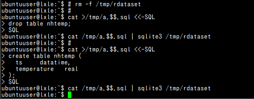

テーブルの作成

◆ bash プログラム

#!/bin/bash

cat >/tmp/a.$$.r <<-RCOMMAND
  library(stats)
  library(graphics)
  library(datasets)
  library(ggplot2)
  library(xts)
  library(chron)
  data(nhtemp)
  D <- as.xts(nhtemp)
#
  write.csv(as.data.frame(D), file="/tmp/nhtemp.csv", row.names=TRUE)
RCOMMAND
#
cat /tmp/a.$$.r | R --no-save

cat >/tmp/a.$$.sql <<-SQL
.mode csv
.import /tmp/a.$$.csv nhtemp
vacuum; 
SQL
#
tail -n +2 /tmp/nhtemp.csv > /tmp/a.$$.csv
cat /tmp/a.$$.sql | sqlite3 /tmp/rdataset
# 
echo 'select * from nhtemp limit 10;' | sqlite3 /tmp/rdataset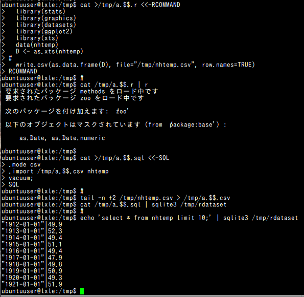

R のプログラム例を用いてプロット

◆ ggplot() を使用 (R プログラム)

  library(ggplot2)
  library(RSQLite)
  library(xts)
  library(chron)

  fetch_table <- function(sqlite3dbname, tablename) {
    drv <- dbDriver("SQLite", max.con = 1)
    conn <- dbConnect(drv, dbname=sqlite3dbname)
    rs <- dbSendQuery( conn, paste("SELECT * from", tablename, ";") )
    T <- fetch(rs, n = -1)
    return(T)
  }

  T <- fetch_table("/tmp/rdataset", "nhtemp")

# 
  table_to_melt <- function(T, tsvec, tsformat) {
    # 先に xts 型に変換しておく
    D <- as.xts( read.zoo( T, tsformat ) )
    # melt(Date, AttrNum, Value). 
    Date <- rep(strptime(tsvec, tsformat, tz=""), ncol(D))
    AttrNum <- rep(1:ncol(D), each=nrow(D))
    Value <- as.numeric(as.vector(D))
    return( data.frame(Date=Date, AttrNum=AttrNum, Value=Value) )
  }
  
  M <- table_to_melt(T, T$ts, "\"%Y-%m-%d\"")

#
  ggplot(M, aes(x=Date, y=Value, colour=factor(AttrNum))) + geom_point(size=2);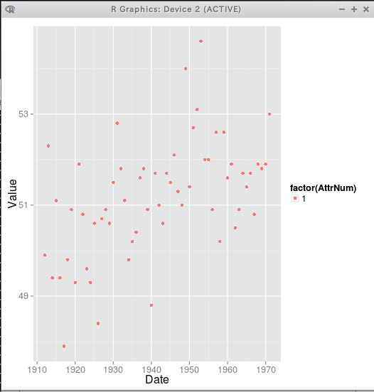

配列

Lai2005fig4

Lai2005fig4 は changepoint パッケージ内の配列データ．

データ源: https://compbio.med.harvard.edu/Supplements/Bioinformatics05b/Profiles/Chrom_7_from40_to65Mb_GBM29.xls

テーブル定義

Lai2005fig4(Spot, CH, POS_start, POS_end, GBM29)

◆ bash プログラム

#!/bin/bash

# rm -f /tmp/rdataset
#
cat >/tmp/a.$$.sql <<-SQL
drop table Lai2005fig4; 
SQL
cat /tmp/a.$$.sql | sqlite3 /tmp/rdataset
#
cat >/tmp/a.$$.sql <<-SQL
create table Lai2005fig4 (
  Spot      integer,
  CH        integer, 
  POS_start integer, 
  POS_end   integer, 
  GBM29     real 
);  
SQL
cat /tmp/a.$$.sql | sqlite3 /tmp/rdataset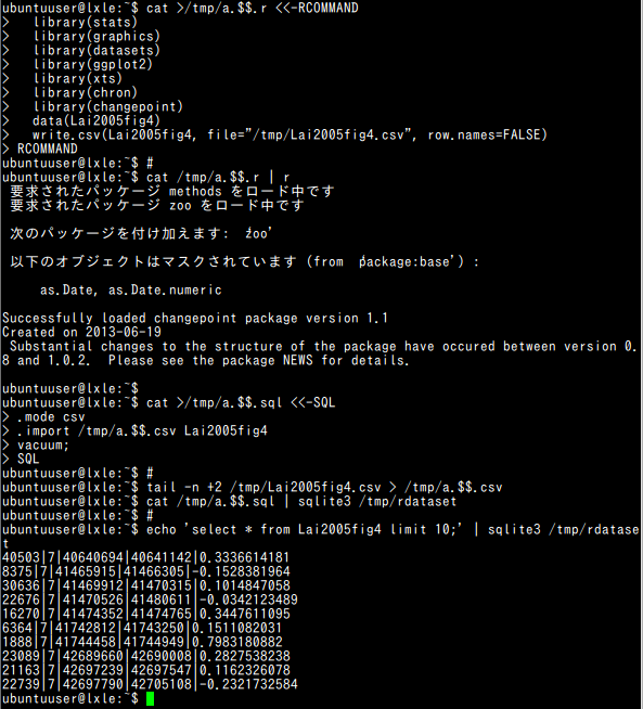

テーブルの作成

◆ bash プログラム

#!/bin/bash

cat >/tmp/a.$$.r <<-RCOMMAND
  library(stats)
  library(graphics)
  library(datasets)
  library(ggplot2)
  library(xts)
  library(chron)
  library(changepoint)
  data(Lai2005fig4)
  write.csv(Lai2005fig4, file="/tmp/Lai2005fig4.csv", row.names=FALSE)  
RCOMMAND
#
cat /tmp/a.$$.r | R --no-save

cat >/tmp/a.$$.sql <<-SQL
.mode csv
.import /tmp/a.$$.csv Lai2005fig4
vacuum; 
SQL
#
tail -n +2 /tmp/Lai2005fig4.csv > /tmp/a.$$.csv
cat /tmp/a.$$.sql | sqlite3 /tmp/rdataset
# 
echo 'select * from Lai2005fig4 limit 10;' | sqlite3 /tmp/rdataset

緯度・経度

wind.loc

ここでの wind.loc は gstat パッケージ内の風向データ

テーブル定義

wind_loc(lat, lon, Station, Code, Latitude, Longitude, MeanWind)

◆ bash プログラム

#!/bin/bash

# rm -f /tmp/rdataset
#
cat >/tmp/a.$$.sql <<-SQL
drop table wind_loc; 
SQL
cat /tmp/a.$$.sql | sqlite3 /tmp/rdataset
#
cat >/tmp/a.$$.sql <<-SQL
create table wind_loc (
  Station   text, 
  Code      text, 
  Latitude  text, 
  Longitude text, 
  MeanWind  real,
  lat       real, 
  lon       real 
);  
SQL
cat /tmp/a.$$.sql | sqlite3 /tmp/rdataset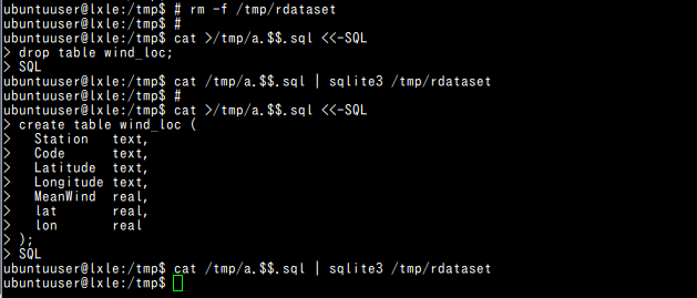

テーブルの作成

◆ bash プログラム

#!/bin/bash

cat >/tmp/a.$$.r <<-RCOMMAND
  library(stats)
  library(graphics)
  library(datasets)
  library(ggplot2)
  library(xts)
  library(chron)
  library(insol)
  library(gstat)
  library(sp)
  data(wind)
  wind.loc\$y = as.numeric(char2dms(as.character(wind.loc[['Latitude']])))
  wind.loc\$x = as.numeric(char2dms(as.character(wind.loc[['Longitude']])))
  coordinates(wind.loc) = ~x+y
  write.csv(wind.loc, file="/tmp/wind.loc.csv", row.names=FALSE)
RCOMMAND
#
cat /tmp/a.$$.r | R --no-save

cat >/tmp/a.$$.sql <<-SQL
.mode csv
.import /tmp/a.$$.csv wind_loc
vacuum; 
SQL
#
tail -n +2 /tmp/wind.loc.csv > /tmp/a.$$.csv
cat /tmp/a.$$.sql | sqlite3 /tmp/rdataset
# 
echo 'select * from wind_loc limit 10;' | sqlite3 /tmp/rdataset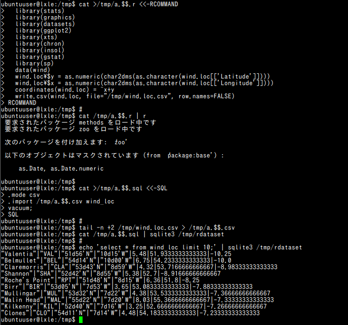

seals

テーブル定義

seals(lat, long, delta_long, delta_lat)

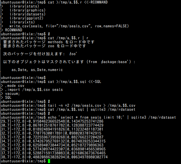
◆ bash プログラム

#!/bin/bash

# rm -f /tmp/rdataset
#
cat >/tmp/a.$$.sql <<-SQL
drop table seals; 
SQL
cat /tmp/a.$$.sql | sqlite3 /tmp/rdataset
#
cat >/tmp/a.$$.sql <<-SQL
create table seals (
  lat        real, 
  long       real, 
  delta_long real, 
  delta_lat  real
);  
SQL
cat /tmp/a.$$.sql | sqlite3 /tmp/rdataset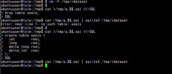

テーブルの作成

◆ bash プログラム

#!/bin/bash

cat >/tmp/a.$$.r <<-RCOMMAND
  library(stats)
  library(graphics)
  library(datasets)
  library(ggplot2)
  library(xts)
  library(chron)
  write.csv(seals, file="/tmp/seals.csv", row.names=FALSE)
RCOMMAND
#
cat /tmp/a.$$.r | R --no-save

cat >/tmp/a.$$.sql <<-SQL
.mode csv
.import /tmp/a.$$.csv seals
vacuum; 
SQL
#
tail -n +2 /tmp/seals.csv > /tmp/a.$$.csv
cat /tmp/a.$$.sql | sqlite3 /tmp/rdataset
# 
echo 'select * from seals limit 10;' | sqlite3 /tmp/rdataset