Ruby で rsruby を用いてグラフ作成するときの各種パラメータ

このページでは， R で 2 次元の散布図を作成する関数である plot() 関数を例として， 各種パラメータを図解で説明する

R システムでのグラフ作成では，各種パラメータを使って，グラフを細かく調整することができる．このページでは， 点と折れ線の重ね合わせ，タイトル付け， x,y値の範囲，対数目盛り，xy比，グラフィックパラメータ（点の色や大きさや形，線の色やスタイルや太さ）を調整する手順を図解で示す．

plot() 関数の実行例

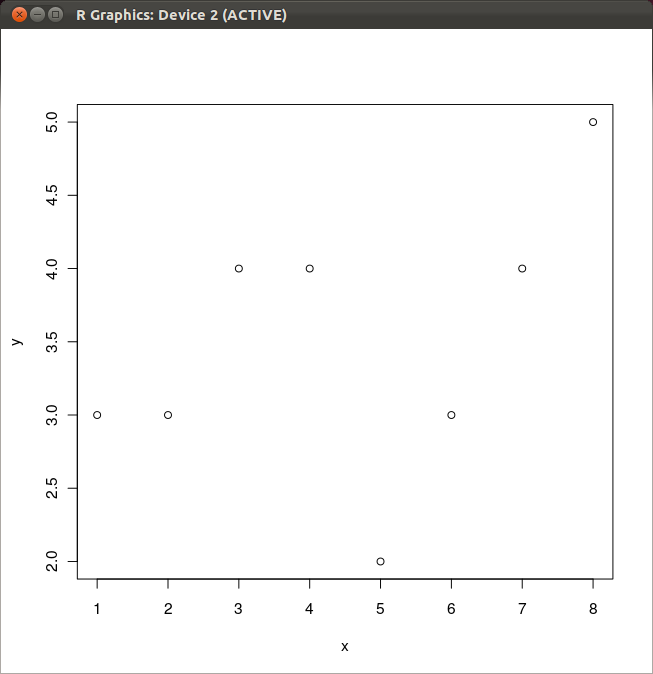
まずは，plot() 関数を使い，x, y 値を指定しての散布図の作成を行う．

x 値を格納したベクトル，y 値を格納したベクトルを引数として plot() 関数を使うと，散布図が描かれます．

◆ Ubuntu の場合の実行手順例

export R_HOME=/usr/lib/R
irb -Ku
require 'rubygems'
require 'rsruby'
T = { "x"=>[1, 2, 3, 4, 5, 6, 7, 8], "y"=>[3, 3, 4, 4, 2, 3, 4, 5] }
r = RSRuby::instance
r.eval_R(<<-RCOMMAND)
     x <- matrix( c( #{T["x"].join(",")} ), 1, #{T["x"].size} )
     y <- matrix( c( #{T["y"].join(",")} ), 1, #{T["y"].size} )
     plot( x, y )
RCOMMAND

種々の散布図

折れ線

◆ Ubuntu の場合の実行手順例

export R_HOME=/usr/lib/R
irb -Ku
require 'rubygems'
require 'rsruby'
T = { "x"=>[1, 2, 3, 4, 5, 6, 7, 8], "y"=>[3, 3, 4, 4, 2, 3, 4, 5] }
r = RSRuby::instance
r.eval_R(<<-RCOMMAND)
     x <- matrix( c( #{T["x"].join(",")} ), 1, #{T["x"].size} )
     y <- matrix( c( #{T["y"].join(",")} ), 1, #{T["y"].size} )
     plot( x, y, type="l" );
RCOMMAND

点と折れ線（点と折れ線が重ならない）

export R_HOME=/usr/lib/R
irb -Ku
require 'rubygems'
require 'rsruby'
T = { "x"=>[1, 2, 3, 4, 5, 6, 7, 8], "y"=>[3, 3, 4, 4, 2, 3, 4, 5] }
r = RSRuby::instance
r.eval_R(<<-RCOMMAND)
     x <- matrix( c( #{T["x"].join(",")} ), 1, #{T["x"].size} )
     y <- matrix( c( #{T["y"].join(",")} ), 1, #{T["y"].size} )
     plot( x, y, type="b" );
RCOMMAND

折れ線（「点」があると思って，折れ線が「点」と重ならないように）

export R_HOME=/usr/lib/R
irb -Ku
require 'rubygems'
require 'rsruby'
T = { "x"=>[1, 2, 3, 4, 5, 6, 7, 8], "y"=>[3, 3, 4, 4, 2, 3, 4, 5] }
r = RSRuby::instance
r.eval_R(<<-RCOMMAND)
     x <- matrix( c( #{T["x"].join(",")} ), 1, #{T["x"].size} )
     y <- matrix( c( #{T["y"].join(",")} ), 1, #{T["y"].size} )
     plot( x, y, type="c" );
RCOMMAND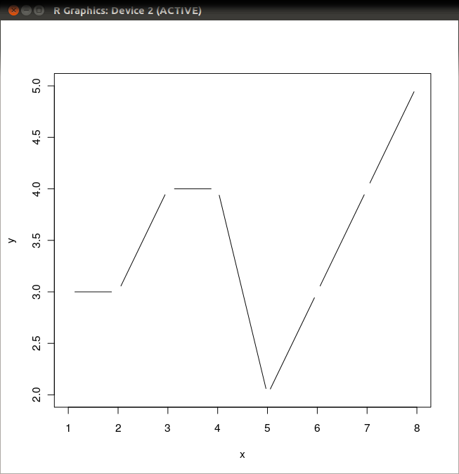

点と折れ線の重ね合わせ

export R_HOME=/usr/lib/R
irb -Ku
require 'rubygems'
require 'rsruby'
T = { "x"=>[1, 2, 3, 4, 5, 6, 7, 8], "y"=>[3, 3, 4, 4, 2, 3, 4, 5] }
r = RSRuby::instance
r.eval_R(<<-RCOMMAND)
     x <- matrix( c( #{T["x"].join(",")} ), 1, #{T["x"].size} )
     y <- matrix( c( #{T["y"].join(",")} ), 1, #{T["y"].size} )
     plot( x, y, type="o" );
RCOMMAND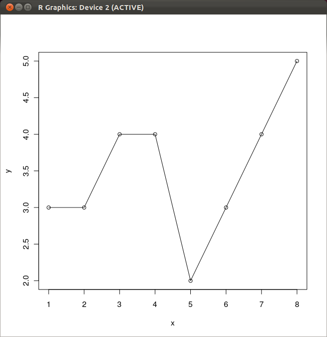

タイトル付け

メインタイトルとサブタイトル

main と sub を使用．メインタイトルはグラフの上に，サブタイトルはグラフの下に書かれる．

export R_HOME=/usr/lib/R
irb -Ku
require 'rubygems'
require 'rsruby'
T = { "x"=>[1, 2, 3, 4, 5, 6, 7, 8], "y"=>[3, 3, 4, 4, 2, 3, 4, 5] }
r = RSRuby::instance
r.eval_R(<<-RCOMMAND)
     x <- matrix( c( #{T["x"].join(",")} ), 1, #{T["x"].size} )
     y <- matrix( c( #{T["y"].join(",")} ), 1, #{T["y"].size} )
     plot( x, y, xlab="x軸のタイトル", sub="y軸のタイトル" )
RCOMMAND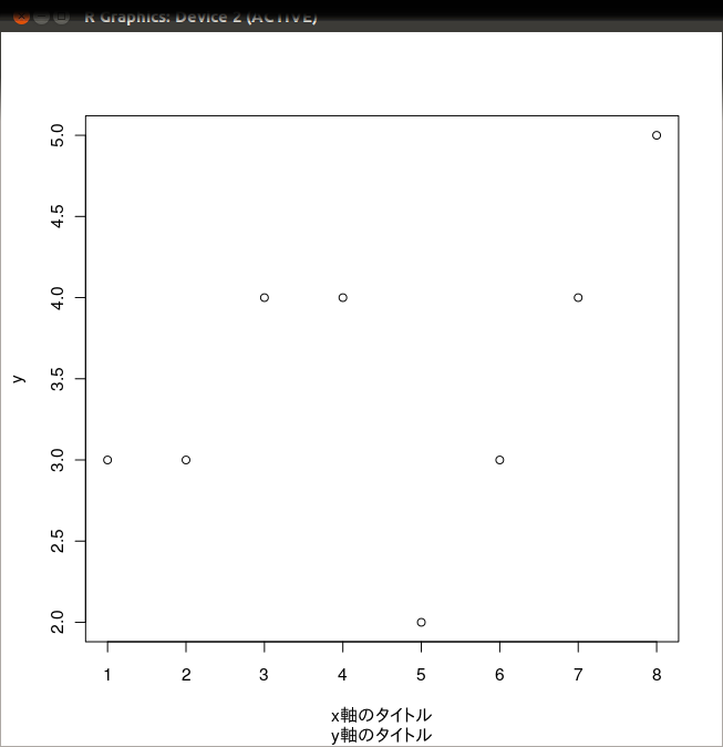

x 軸のタイトルとy 軸のタイトル

xlab と ylab を使用．

export R_HOME=/usr/lib/R
irb -Ku
require 'rubygems'
require 'rsruby'
T = { "x"=>[1, 2, 3, 4, 5, 6, 7, 8], "y"=>[3, 3, 4, 4, 2, 3, 4, 5] }
r = RSRuby::instance
r.eval_R(<<-RCOMMAND)
     x <- matrix( c( #{T["x"].join(",")} ), 1, #{T["x"].size} )
     y <- matrix( c( #{T["y"].join(",")} ), 1, #{T["y"].size} )
     plot( x, y, xlab="x軸のタイトル", ylab="y軸のタイトル" )
RCOMMAND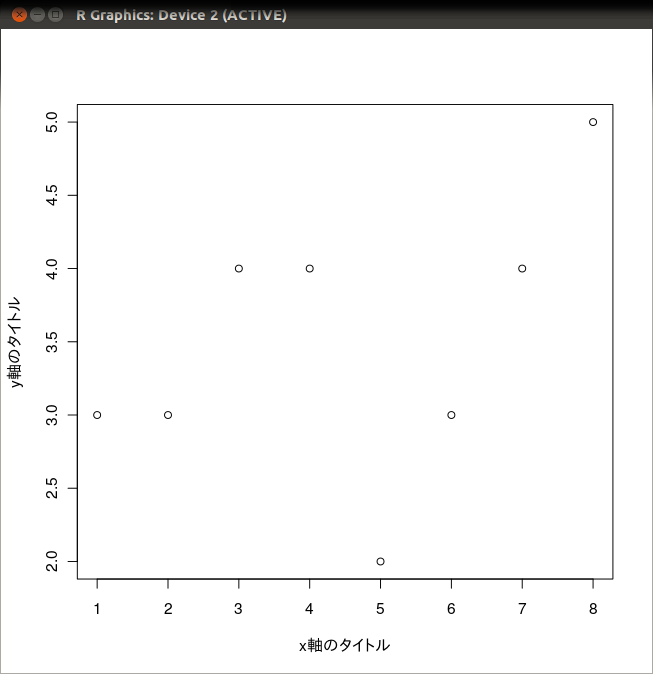

タイトルとして数式を表示

expression オブジェクトを使う．

export R_HOME=/usr/lib/R
irb -Ku
require 'rubygems'
require 'rsruby'
r = RSRuby::instance
r.eval_R(<<-RCOMMAND)
    X <- seq(1, 5, length=100)
    Y <- exp(-.5 * log( X^2 ) )
    plot(X, Y, type="o", xlab="x", ylab=expression(e^{-frac(1,2) * {log[10](x)}^2}) )
RCOMMAND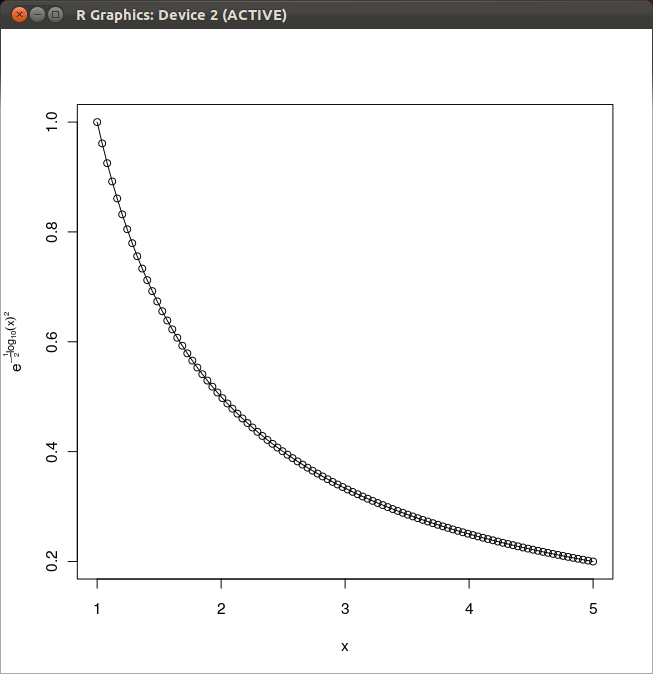

x,y値の範囲，対数目盛り，xy比

x,y値の範囲

export R_HOME=/usr/lib/R
irb -Ku
require 'rubygems'
require 'rsruby'
T = { "x"=>[1, 2, 3, 4, 5, 6, 7, 8], "y"=>[3, 3, 4, 4, 2, 3, 4, 5] }
r = RSRuby::instance
r.eval_R(<<-RCOMMAND)
     x <- matrix( c( #{T["x"].join(",")} ), 1, #{T["x"].size} )
     y <- matrix( c( #{T["y"].join(",")} ), 1, #{T["y"].size} )
     plot( x, y, xlim=c(0,10), ylim=c(0,6) )
RCOMMAND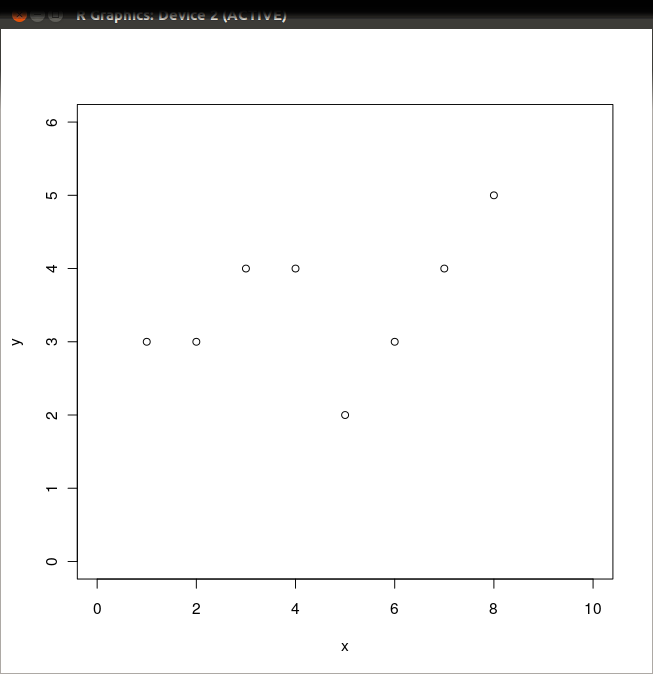

x軸を対数目盛り

export R_HOME=/usr/lib/R
irb -Ku
require 'rubygems'
require 'rsruby'
T = { "x"=>[1, 2, 3, 4, 5, 6, 7, 8], "y"=>[3, 3, 4, 4, 2, 3, 4, 5] }
r = RSRuby::instance
r.eval_R(<<-RCOMMAND)
     x <- matrix( c( #{T["x"].join(",")} ), 1, #{T["x"].size} )
     y <- matrix( c( #{T["y"].join(",")} ), 1, #{T["y"].size} )
     plot( x, y, log="x" )
RCOMMAND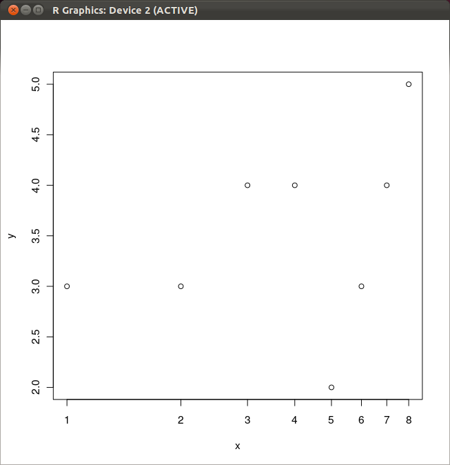

y軸を対数目盛り

export R_HOME=/usr/lib/R
irb -Ku
require 'rubygems'
require 'rsruby'
T = { "x"=>[1, 2, 3, 4, 5, 6, 7, 8], "y"=>[3, 3, 4, 4, 2, 3, 4, 5] }
r = RSRuby::instance
r.eval_R(<<-RCOMMAND)
     x <- matrix( c( #{T["x"].join(",")} ), 1, #{T["x"].size} )
     y <- matrix( c( #{T["y"].join(",")} ), 1, #{T["y"].size} )
     plot( x, y, log="y" )
RCOMMAND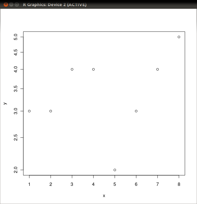

x, y軸を対数目盛り

export R_HOME=/usr/lib/R
irb -Ku
require 'rubygems'
require 'rsruby'
T = { "x"=>[1, 2, 3, 4, 5, 6, 7, 8], "y"=>[3, 3, 4, 4, 2, 3, 4, 5] }
r = RSRuby::instance
r.eval_R(<<-RCOMMAND)
     x <- matrix( c( #{T["x"].join(",")} ), 1, #{T["x"].size} )
     y <- matrix( c( #{T["y"].join(",")} ), 1, #{T["y"].size} )
     plot( x, y, log="xy" )
RCOMMAND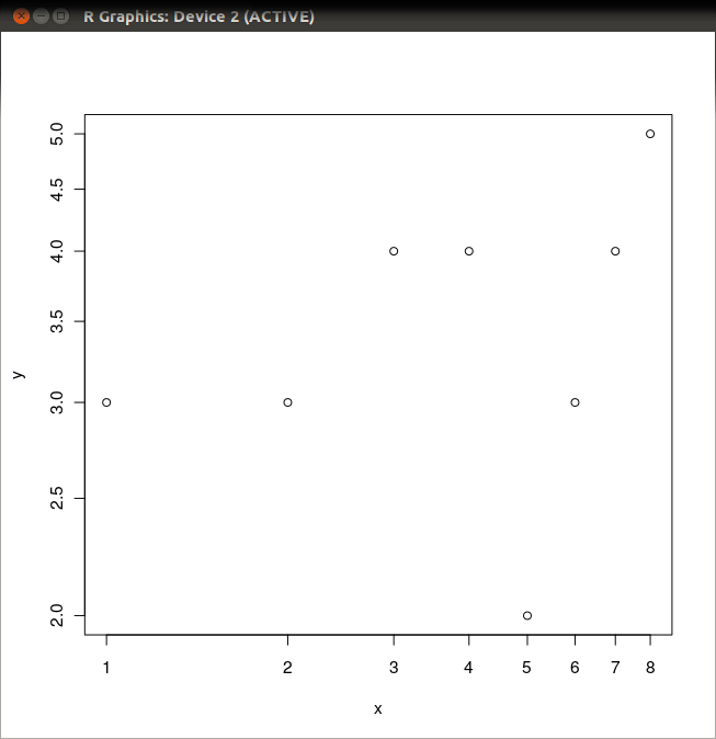

補助線 （格子状）

export R_HOME=/usr/lib/R
irb -Ku
require 'rubygems'
require 'rsruby'
T = { "x"=>[1, 2, 3, 4, 5, 6, 7, 8], "y"=>[3, 3, 4, 4, 2, 3, 4, 5] }
r = RSRuby::instance
r.eval_R(<<-RCOMMAND)
     x <- matrix( c( #{T["x"].join(",")} ), 1, #{T["x"].size} )
     y <- matrix( c( #{T["y"].join(",")} ), 1, #{T["y"].size} )
     plot( x, y, panel.first=grid(8,8) )
RCOMMAND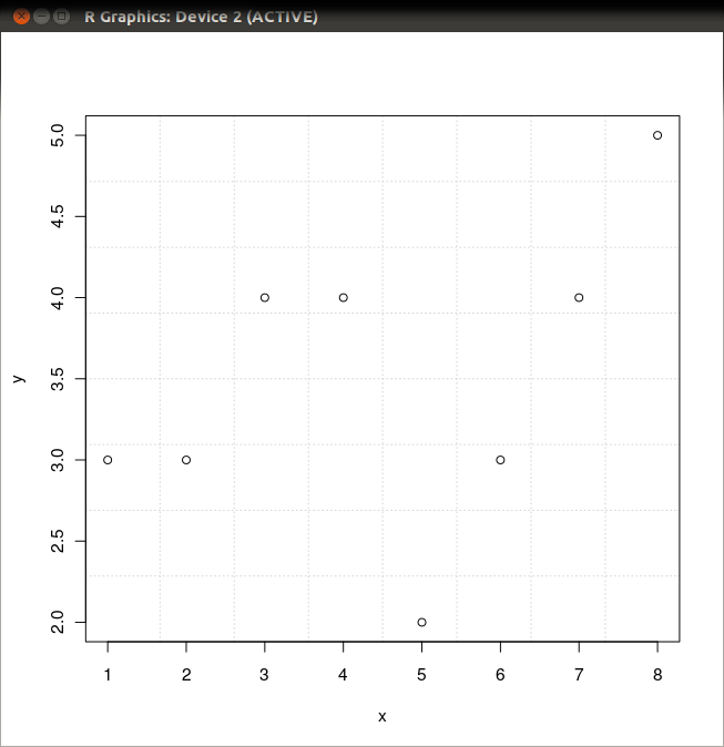

補助線 （なめらかな折れ線）

export R_HOME=/usr/lib/R
irb -Ku
require 'rubygems'
require 'rsruby'
T = { "x"=>[1, 2, 3, 4, 5, 6, 7, 8], "y"=>[3, 3, 4, 4, 2, 3, 4, 5] }
r = RSRuby::instance
r.eval_R(<<-RCOMMAND)
     x <- matrix( c( #{T["x"].join(",")} ), 1, #{T["x"].size} )
     y <- matrix( c( #{T["y"].join(",")} ), 1, #{T["y"].size} )
     plot( x, y, panel.first = lines(stats::lowess( x, y ), lty="dashed") )
RCOMMAND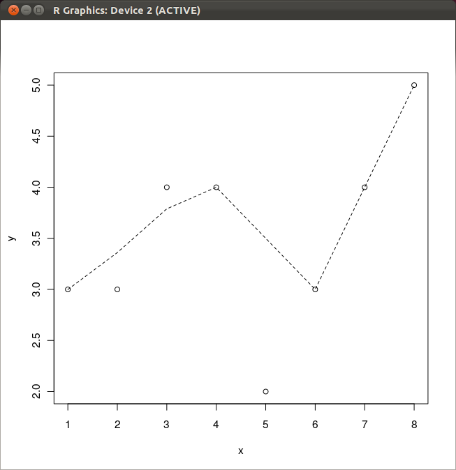

xy比

export R_HOME=/usr/lib/R
irb -Ku
require 'rubygems'
require 'rsruby'
T = { "x"=>[1, 2, 3, 4, 5, 6, 7, 8], "y"=>[3, 3, 4, 4, 2, 3, 4, 5] }
r = RSRuby::instance
r.eval_R(<<-RCOMMAND)
     x <- matrix( c( #{T["x"].join(",")} ), 1, #{T["x"].size} )
     y <- matrix( c( #{T["y"].join(",")} ), 1, #{T["y"].size} )
     plot( x, y, asp="0.4" )
RCOMMAND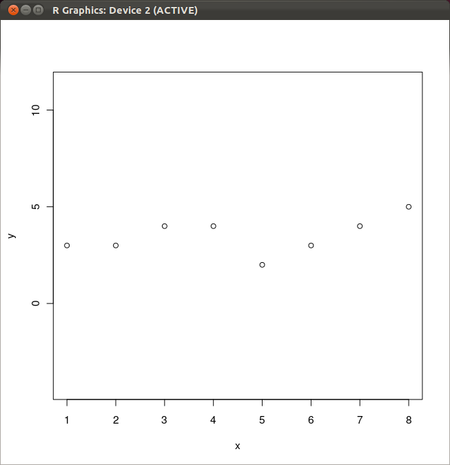

グラフィックパラメータ

点や線の色

export R_HOME=/usr/lib/R
irb -Ku
require 'rubygems'
require 'rsruby'
T = { "x"=>[1, 2, 3, 4, 5, 6, 7, 8], "y"=>[3, 3, 4, 4, 2, 3, 4, 5] }
r = RSRuby::instance
r.eval_R(<<-RCOMMAND)
     x <- matrix( c( #{T["x"].join(",")} ), 1, #{T["x"].size} )
     y <- matrix( c( #{T["y"].join(",")} ), 1, #{T["y"].size} )
     plot( x, y, type="o", col="red" )
RCOMMAND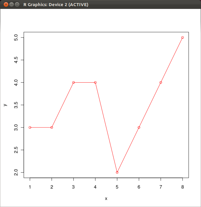

点の四角形に変更

export R_HOME=/usr/lib/R
irb -Ku
require 'rubygems'
require 'rsruby'
T = { "x"=>[1, 2, 3, 4, 5, 6, 7, 8], "y"=>[3, 3, 4, 4, 2, 3, 4, 5] }
r = RSRuby::instance
r.eval_R(<<-RCOMMAND)
     x <- matrix( c( #{T["x"].join(",")} ), 1, #{T["x"].size} )
     y <- matrix( c( #{T["y"].join(",")} ), 1, #{T["y"].size} )
     plot( x, y, type="o", pch = 0 )
RCOMMAND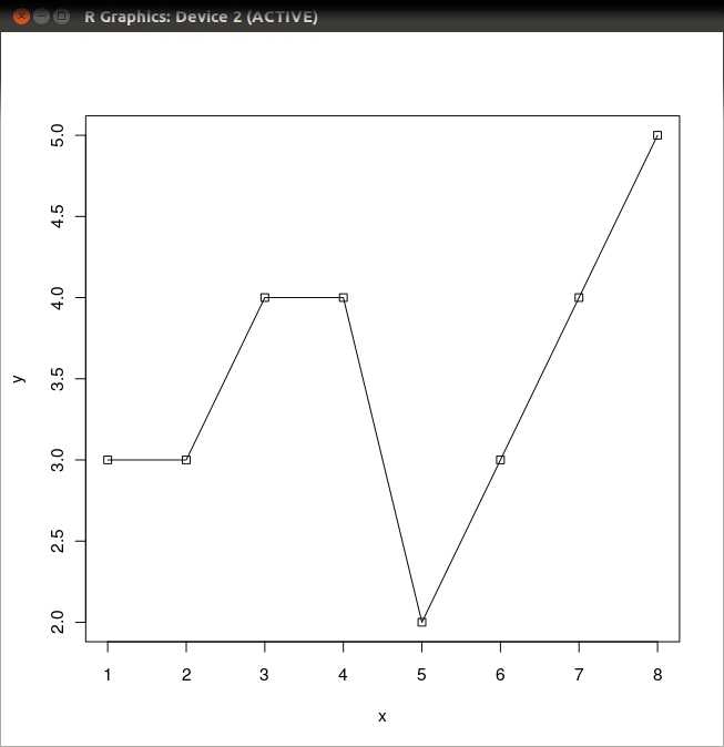

点の大きさ

export R_HOME=/usr/lib/R
irb -Ku
require 'rubygems'
require 'rsruby'
T = { "x"=>[1, 2, 3, 4, 5, 6, 7, 8], "y"=>[3, 3, 4, 4, 2, 3, 4, 5] }
r = RSRuby::instance
r.eval_R(<<-RCOMMAND)
     x <- matrix( c( #{T["x"].join(",")} ), 1, #{T["x"].size} )
     y <- matrix( c( #{T["y"].join(",")} ), 1, #{T["y"].size} )
     plot( x, y, type="o", cex=4 )
RCOMMAND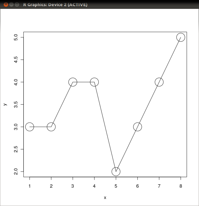

線のスタイル（破線）

export R_HOME=/usr/lib/R
irb -Ku
require 'rubygems'
require 'rsruby'
T = { "x"=>[1, 2, 3, 4, 5, 6, 7, 8], "y"=>[3, 3, 4, 4, 2, 3, 4, 5] }
r = RSRuby::instance
r.eval_R(<<-RCOMMAND)
     x <- matrix( c( #{T["x"].join(",")} ), 1, #{T["x"].size} )
     y <- matrix( c( #{T["y"].join(",")} ), 1, #{T["y"].size} )
     plot( x, y, type="o", lty=2 )
RCOMMAND

線のスタイル（点線）

export R_HOME=/usr/lib/R
irb -Ku
require 'rubygems'
require 'rsruby'
T = { "x"=>[1, 2, 3, 4, 5, 6, 7, 8], "y"=>[3, 3, 4, 4, 2, 3, 4, 5] }
r = RSRuby::instance
r.eval_R(<<-RCOMMAND)
     x <- matrix( c( #{T["x"].join(",")} ), 1, #{T["x"].size} )
     y <- matrix( c( #{T["y"].join(",")} ), 1, #{T["y"].size} )
     plot( x, y, type="o", lty=3 )
RCOMMAND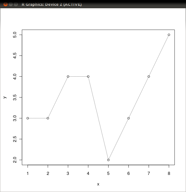

線のスタイル（破線）

export R_HOME=/usr/lib/R
irb -Ku
require 'rubygems'
require 'rsruby'
T = { "x"=>[1, 2, 3, 4, 5, 6, 7, 8], "y"=>[3, 3, 4, 4, 2, 3, 4, 5] }
r = RSRuby::instance
r.eval_R(<<-RCOMMAND)
     x <- matrix( c( #{T["x"].join(",")} ), 1, #{T["x"].size} )
     y <- matrix( c( #{T["y"].join(",")} ), 1, #{T["y"].size} )
     plot( x, y, type="o", lty=5 )
RCOMMAND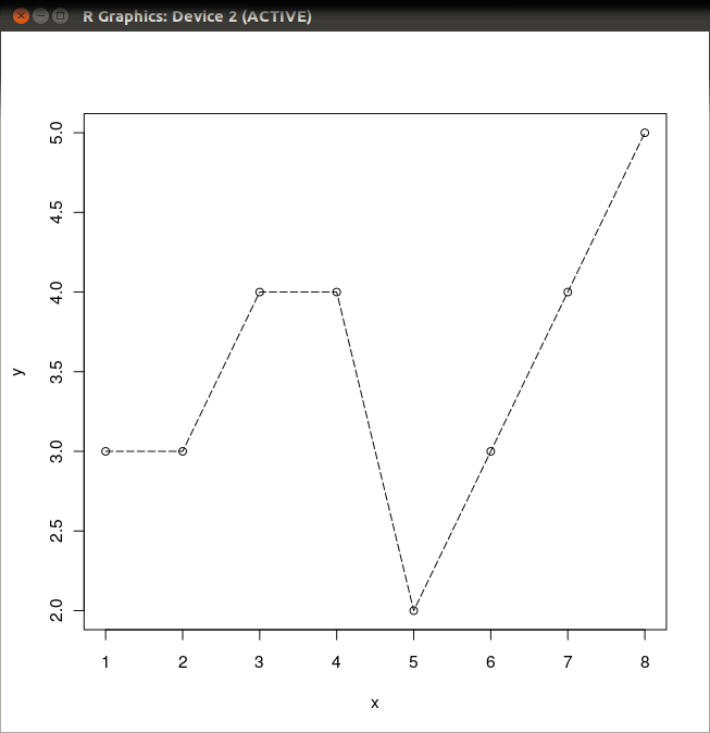

線のスタイル（破線）

export R_HOME=/usr/lib/R
irb -Ku
require 'rubygems'
require 'rsruby'
T = { "x"=>[1, 2, 3, 4, 5, 6, 7, 8], "y"=>[3, 3, 4, 4, 2, 3, 4, 5] }
r = RSRuby::instance
r.eval_R(<<-RCOMMAND)
     x <- matrix( c( #{T["x"].join(",")} ), 1, #{T["x"].size} )
     y <- matrix( c( #{T["y"].join(",")} ), 1, #{T["y"].size} )
     plot( x, y, type="o", lty=5 )
RCOMMAND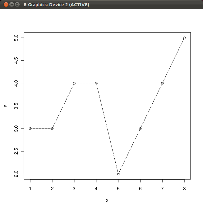

線の太さ

export R_HOME=/usr/lib/R
irb -Ku
require 'rubygems'
require 'rsruby'
T = { "x"=>[1, 2, 3, 4, 5, 6, 7, 8], "y"=>[3, 3, 4, 4, 2, 3, 4, 5] }
r = RSRuby::instance
r.eval_R(<<-RCOMMAND)
     x <- matrix( c( #{T["x"].join(",")} ), 1, #{T["x"].size} )
     y <- matrix( c( #{T["y"].join(",")} ), 1, #{T["y"].size} )
     plot( x, y, type="o", lwd=4 )
RCOMMAND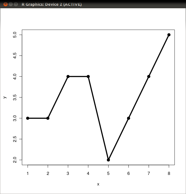

（参考）plot() 関数のヘルプ

Usage

plot(x, y, ...)

Arguments

x the coordinates of points in the plot.
x the coordinates of points in the plot. Alternatively, a single plotting structure, function or any R object with a plot method can be provided.
y the y coordinates of points in the plot, optional if x is an appropriate structure.
... Arguments to be passed to methods, such as graphical parameters (see par). Many methods will accept the following arguments:
- type what type of plot should be drawn. Possible types are
  - "p" for points,
  - "l" for lines,
  - "b" for both,
  - "c" for the lines part alone of "b",
  - "o" for both ‘overplotted’,
  - "h" for ‘histogram’ like (or ‘high-density’) vertical lines,
  - "s" for stair steps,
  - "S" for other steps, see ‘Details’ below,
  - "n" for no plotting.
  All other types give a warning or an error; using, e.g., type = "punkte" being equivalent to type = "p" for S compatibility.
- main an overall title for the plot: see title.
- sub a sub title for the plot: see title.
- xlab a title for the x axis: see title.
- ylab a title for the y axis: see title.
- asp the y/x aspect ratio, see plot.window.

See Also plot.default, plot.formula and other methods; points, lines, par.

（参考）plot.default() 関数のヘルプ

Usage

plot(x, y = NULL, type = "p",  xlim = NULL, ylim = NULL,
     log = "", main = NULL, sub = NULL, xlab = NULL, ylab = NULL,
     ann = par("ann"), axes = TRUE, frame.plot = axes,
     panel.first = NULL, panel.last = NULL, asp = NA, ...)

Arguments

x, y the x and y arguments provide the x and y coordinates for the plot. Any reasonable way of defining the coordinates is acceptable. See the function xy.coords for details. If supplied separately, they must be of the same length.
type 1-character string giving the type of plot desired. The following values are possible, for details, see plot: "p" for points, "l" for lines, "o" for overplotted points and lines, "b", "c") for (empty if "c") points joined by lines, "s" and "S" for stair steps and "h" for histogram-like vertical lines. Finally, "n" does not produce any points or lines.
xlim the x limits (x1, x2) of the plot. Note that x1 > x2 is allowed and leads to a ‘reversed axis’.
ylim the y limits of the plot.
log a character string which contains "x" if the x axis is to be logarithmic, "y" if the y axis is to be logarithmic and "xy" or "yx" if both axes are to be logarithmic.
main a main title for the plot, see also title.
sub a sub title for the plot.
xlab a label for the x axis, defaults to a description of x.
ylab a label for the y axis, defaults to a description of y.
ann a logical value indicating whether the default annotation (title and x and y axis labels) should appear on the plot.
axes a logical value indicating whether both axes should be drawn on the plot. Use graphical parameter "xaxt" or "yaxt" to suppress just one of the axes.
frame.plot a logical indicating whether a box should be drawn around the plot.
panel.first an expression to be evaluated after the plot axes are set up but before any plotting takes place. This can be useful for drawing background grids or scatterplot smooths.
panel.last an expression to be evaluated after plotting has taken place.
asp the y/x aspect ratio, see plot.window.
... other graphical parameters (see par and section ‘Details’ below).

Usage

Commonly used graphical parameters are:

col The colors for lines and points. Multiple colors can be specified so that each point can be given its own color. If there are fewer colors than points they are recycled in the standard fashion. Lines will all be plotted in the first colour specified.
bg a vector of background colors for open plot symbols, see points. Note: this is not the same setting as par("bg").
pch a vector of plotting characters or symbols: see points.
cex a numerical vector giving the amount by which plotting characters and symbols should be scaled relative to the default. This works as a multiple of par("cex"). NULL and NA are equivalent to 1.0. Note that this does not affect annotation: see below.
lty the line type, see par.
cex.main, col.lab, font.sub, etc settings for main- and sub-title and axis annotation, see title and par.
lwd the line width, see par.

References

Becker, R. A., Chambers, J. M. and Wilks, A. R. (1988) The New S Language. Wadsworth & Brooks/Cole.
Cleveland, W. S. (1985) The Elements of Graphing Data. Monterey, CA: Wadsworth.
Murrell, P. (2005) R Graphics. Chapman & Hall/CRC Press.