TensorFlow のパイプラインを用いたMNIST データセットによる学習と分類(TensorFlow データセット,TensorFlow,Python を使用)(Windows 上,Google Colaboratroy の両方を記載)
ニューラルネットワークによるデータの分類を行う. ここでの分類は,データから,そのラベル(クラス名)を求めるもの. 分類のために,教師データを用いてニューラルネットワークの学習を行う.
このページでは,TensorFlow データセットの中の MNIST データセットを用いて,TensorFlow での学習を行うととも に,データの分類も行う.
データセットの利用条件は利用者で確認すること. このページの内容は, https://www.tensorflow.org/datasets/keras_example による.
【目次】
- Google Colaboratory での実行
- Windows での実行
- MNIST データセットのロード
- MNIST データセットの確認
- Keras を用いたニューラルネットワークの作成
- ニューラルネットワークの学習と検証
【サイト内の関連ページ】
【関連する外部ページ】
- TensorFlow データセットカタログの MNIST のページ: https://www.tensorflow.org/datasets/catalog/mnist
- TensorFlow データセットの URL: https://www.tensorflow.org/datasets
- TensorFlow データセットの一覧の URL: https://www.tensorflow.org/datasets/catalog/overview
- TensorFlow のクイックスタートのページ: https://www.tensorflow.org/tutorials/quickstart/advanced
1. Google Colaboratory での実行
Google Colaboratory のページ:
次のリンクをクリックすると,Google Colaboratory のノートブックが開く. そして,Google アカウントでログインすると,Google Colaboratory のノートブック内のコード等を編集したり再実行したりができる.編集した場合でも,他の人に影響が出たりということはない.そして,編集後のものを,各自の Google ドライブ内に保存することもできる.
https://colab.research.google.com/drive/1QvEEivjsqTK3s1QV5yn-COo-HavIlO2U?usp=sharing
2. Windows での実行
Python 3.12 のインストール
インストール済みの場合は実行不要。
管理者権限でコマンドプロンプトを起動(手順:Windowsキーまたはスタートメニュー > cmd と入力 > 右クリック > 「管理者として実行」)し、以下を実行する。管理者権限は、wingetの--scope machineオプションでシステム全体にソフトウェアをインストールするために必要である。
REM Python をシステム領域にインストール
winget install --scope machine --id Python.Python.3.12 -e --silent --accept-source-agreements --accept-package-agreements
REM Python のパス設定
set "PYTHON_PATH=C:\Program Files\Python312"
set "PYTHON_SCRIPTS_PATH=C:\Program Files\Python312\Scripts"
echo "%PATH%" | find /i "%PYTHON_PATH%" >nul
if errorlevel 1 setx PATH "%PATH%;%PYTHON_PATH%" /M >nul
echo "%PATH%" | find /i "%PYTHON_SCRIPTS_PATH%" >nul
if errorlevel 1 setx PATH "%PATH%;%PYTHON_SCRIPTS_PATH%" /M >nul【関連する外部ページ】
Python の公式ページ: https://www.python.org/
AI エディタ Windsurf のインストール
Pythonプログラムの編集・実行には、AI エディタの利用を推奨する。ここでは,Windsurfのインストールを説明する。
管理者権限でコマンドプロンプトを起動(手順:Windowsキーまたはスタートメニュー > cmd と入力 > 右クリック > 「管理者として実行」)し、以下を実行して、Windsurfをシステム全体にインストールする。管理者権限は、wingetの--scope machineオプションでシステム全体にソフトウェアをインストールするために必要となる。
winget install --scope machine --id Codeium.Windsurf -e --silent --accept-source-agreements --accept-package-agreements【関連する外部ページ】
Windsurf の公式ページ: https://windsurf.com/
Gitのインストール
管理者権限でコマンドプロンプトを起動(手順:Windowsキーまたはスタートメニュー > cmd と入力 > 右クリック > 「管理者として実行」)し、以下を実行する。管理者権限は、wingetの--scope machineオプションでシステム全体にソフトウェアをインストールするために必要となる。
REM Git をシステム領域にインストール
winget install --scope machine --id Git.Git -e --silent --accept-source-agreements --accept-package-agreements
REM Git のパス設定
set "GIT_PATH=C:\Program Files\Git\cmd"
if exist "%GIT_PATH%" (
    echo "%PATH%" | find /i "%GIT_PATH%" >nul
    if errorlevel 1 setx PATH "%PATH%;%GIT_PATH%" /M >nul
)
7-Zip のインストール
管理者権限でコマンドプロンプトを起動(手順:Windowsキーまたはスタートメニュー > cmd と入力 > 右クリック > 「管理者として実行」)し、以下を実行する。管理者権限は、wingetの--scope machineオプションでシステム全体にソフトウェアをインストールするために必要となる。
REM 7-Zip をシステム領域にインストール
winget install --scope machine --id 7zip.7zip -e --silent
REM 7-Zip のパス設定
set "SEVENZIP_PATH=C:\Program Files\7-Zip"
if exist "%SEVENZIP_PATH%" (
    echo "%PATH%" | find /i "%SEVENZIP_PATH%" >nul
    if errorlevel 1 setx PATH "%PATH%;%SEVENZIP_PATH%" /M >nul
)
Visual Studio 2022 Build Toolsとランタイムのインストール
管理者権限でコマンドプロンプトを起動(手順:Windowsキーまたはスタートメニュー > cmd と入力 > 右クリック > 「管理者として実行」)し、以下を実行する。管理者権限は、wingetの--scope machineオプションでシステム全体にソフトウェアをインストールするために必要である。
REM Visual Studio 2022 Build Toolsとランタイムのインストール
winget install --scope machine --wait --accept-source-agreements --accept-package-agreements Microsoft.VisualStudio.2022.BuildTools Microsoft.VCRedist.2015+.x64

REM インストーラーとインストールパスの設定
set VS_INSTALLER="C:\Program Files (x86)\Microsoft Visual Studio\Installer\vs_installer.exe"
set VS_PATH="C:\Program Files (x86)\Microsoft Visual Studio\2022\BuildTools"

REM C++開発ワークロードのインストール(次のコマンドは全体で1行である)
%VS_INSTALLER% modify --installPath %VS_PATH% --add Microsoft.VisualStudio.Workload.VCTools --add Microsoft.VisualStudio.Component.VC.Tools.x86.x64 --add Microsoft.VisualStudio.Component.Windows11SDK.22621 --includeRecommended --quiet --norestart
NVIDIA ドライバのインストール(Windows 上)
NVIDIA ドライバとは
NVIDIA ドライバは,NVIDIA製GPUをWindowsシステム上で適切に動作させるための基盤となるソフトウェアです.このドライバをインストールすることにより,GPUの性能を最大限に引き出し,グラフィックス処理はもちろん,CUDAを利用したAI関連アプリケーションなどの計算速度を向上させることが期待できます.
ドライバは通常、NVIDIA公式サイトからダウンロードするか、NVIDIA GeForce Experienceソフトウェアを通じてインストール・更新します。
公式サイト: https://www.nvidia.co.jp/Download/index.aspx?lang=jp
【サイト内の関連ページ】
- (再掲) NVIDIA グラフィックス・ボードの確認
インストールするドライバを選択するために、まずご使用のPCに搭載されているNVIDIAグラフィックス・ボードの種類を確認します。(確認済みであれば、この手順は不要です。) Windows のコマンドプロンプトで次のコマンドを実行します。
wmic path win32_VideoController get name
- NVIDIA ドライバのダウンロード
確認したグラフィックス・ボードのモデル名と、お使いのWindowsのバージョン(例: Windows 11, Windows 10 64-bit)に対応するドライバを、以下のNVIDIA公式サイトからダウンロードします.
https://www.nvidia.co.jp/Download/index.aspx?lang=jp
サイトの指示に従い、製品タイプ、製品シリーズ、製品ファミリー、OS、言語などを選択して検索し、適切なドライバ(通常は最新のGame Ready ドライバまたはStudio ドライバ)をダウンロードします。
- ドライバのインストール
ダウンロードしたインストーラー(.exeファイル)を実行し、画面の指示に従ってインストールを進めます。「カスタムインストール」を選択すると、インストールするコンポーネント(ドライバ本体、GeForce Experience、PhysXなど)を選ぶことができます。通常は「高速(推奨)」で問題ありません。
インストール完了後、システムの再起動を求められる場合があります。
- CUDA対応のNVIDIA GPU。
- 対応するNVIDIA ドライバ。
- サポートされているバージョンのC++コンパイラ (Visual StudioまたはBuild Toolsをインストール済み)。
- Windows では,NVIDIA CUDA ツールキットのインストール中は,予期せぬ問題を避けるため、なるべく他のアプリケーションは終了しておくことが推奨されます。
- インストール後に環境変数が正しく設定されているか確認することが重要です。
- NVIDIA CUDA ツールキットのアーカイブの公式ページ: https://developer.nvidia.com/cuda-toolkit-archive (他のバージョンが必要な場合)
- NVIDIA CUDA ツールキット の公式ドキュメント: https://docs.nvidia.com/cuda/index.html
- NVIDIA CUDA ツールキットのインストールに関する,NVIDIA CUDA Installation Guide for Windows: https://docs.nvidia.com/cuda/cuda-installation-guide-windows/index.html
- (再掲) 他のウィンドウを閉じる:インストール中のコンフリクトを避けるため、可能な限り他のアプリケーションを終了します。
- Windows で,コマンドプロンプトを管理者権限で起動します。
-
wingetコマンドで CUDA 11.8 をインストールします。以下のコマンドは、(必要であれば)NVIDIA GeForce Experienceと、指定したバージョンのNVIDIA CUDA ツールキット (11.8) をインストールします。また、
CUDA_HOME環境変数を設定します(一部のツールで参照されることがあります)。rem グラフィックボードの確認 (参考) wmic path win32_VideoController get name rem CUDA Toolkit 11.8 のインストール winget install --scope machine Nvidia.CUDA --version 11.8 rem CUDA_HOME 環境変数の設定 (システム環境変数として設定) powershell -command "[System.Environment]::SetEnvironmentVariable(\"CUDA_HOME\", \"C:\Program Files\NVIDIA GPU Computing Toolkit\CUDA\v11.8\", \"Machine\")"
注釈: これは特定のバージョン(11.8)をインストールする例です。他のバージョンをインストールする場合は
--versionオプションを適宜変更してください(例:--version 11.2)。利用可能なバージョンはwinget search Nvidia.CUDAで確認できます。 - (重要) ユーザ環境変数 TEMP の設定(日本語ユーザ名の場合)
Windows のユーザ名に日本語(マルチバイト文字)が含まれている場合、CUDAコンパイラ
nvccが一時ファイルの作成に失敗し、コンパイルが正常に動作しないことがあります(エラーメッセージが表示されない場合もあるため注意が必要です)。この問題を回避するために、ユーザ環境変数TEMPおよびTMPを、ASCII文字のみのパス(例:C:\TEMP)に変更します。管理者権限のコマンドプロンプトで,次のコマンドを実行して
C:\TEMPディレクトリを作成し、ユーザ環境変数TEMPとTMPを設定します。mkdir C:\TEMP powershell -command "[System.Environment]::SetEnvironmentVariable(\"TEMP\", \"C:\TEMP\", \"User\")" powershell -command "[System.Environment]::SetEnvironmentVariable(\"TMP\", \"C:\TEMP\", \"User\")"
この設定は、コマンドプロンプトを再起動するか、Windowsに再サインインした後に有効になります。
- NVIDIA cuDNN の公式ページ(ダウンロードにはDeveloper Programへの登録が必要): https://developer.nvidia.com/cudnn
- NVIDIA Developer Program メンバーシップへの加入: cuDNNのダウンロードには無料のメンバーシップ登録が必要です。
NVIDIA Developer Program の公式ページ: https://developer.nvidia.com/developer-program
- 互換バージョンの選択とダウンロード: インストール済みのCUDAツールキットのバージョン (今回は11.x) に適合するcuDNNのバージョン (今回はv8.9.7) を選択し、Windows用のzipファイルをダウンロードします。
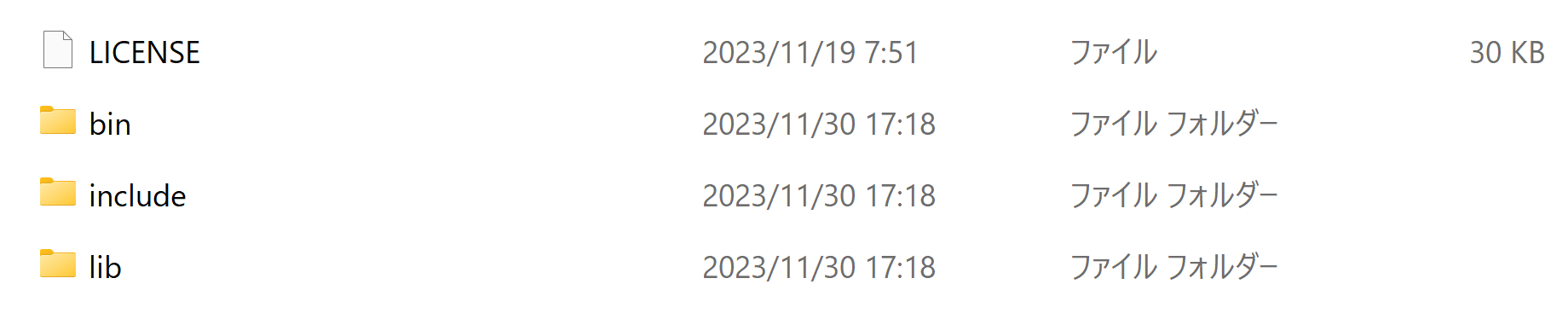
- ファイルの展開と配置: ダウンロードしたzipファイルを展開(解凍)し、中のファイル(
bin,include,libフォルダ内)を、CUDAツールキットのインストールディレクトリにコピーします。 - (オプション) 環境変数の設定: 必要に応じてシステム環境変数
CUDNN_PATHを設定します。 - (必要に応じて) ZLIB DLL のインストール:
zlibwapi.dllが見つからないエラーが発生する場合にインストールします。 - 動作確認: cuDNNライブラリ (
cudnn64_*.dll) にパスが通っているか確認します。 - Windows で,管理者権限でコマンドプロンプトを起動(手順:Windowsキーまたはスタートメニュー >
cmdと入力 > 右クリック > 「管理者として実行」)。 - 次のコマンドを実行
次のコマンドは,zlibをインストールし,パスを通すものである.
cd /d c:%HOMEPATH%
rmdir /s /q zlib
git clone https://github.com/madler/zlib
cd zlib
del CMakeCache.txt
rmdir /s /q CMakeFiles\
cmake . -G "Visual Studio 17 2022" -A x64 -T host=x64 -DCMAKE_INSTALL_PREFIX=c:/zlib
cmake --build . --config RELEASE --target INSTALL
powershell -command "$oldpath = [System.Environment]::GetEnvironmentVariable(\"Path\", \"Machine\"); $oldpath += \";c:\zlib\bin\"; [System.Environment]::SetEnvironmentVariable(\"Path\", $oldpath, \"Machine\")"
powershell -command "[System.Environment]::SetEnvironmentVariable(\"ZLIB_HOME\", \"C:\zlib\", \"Machine\")"
- zlib の公式ページ: https://www.zlib.net/
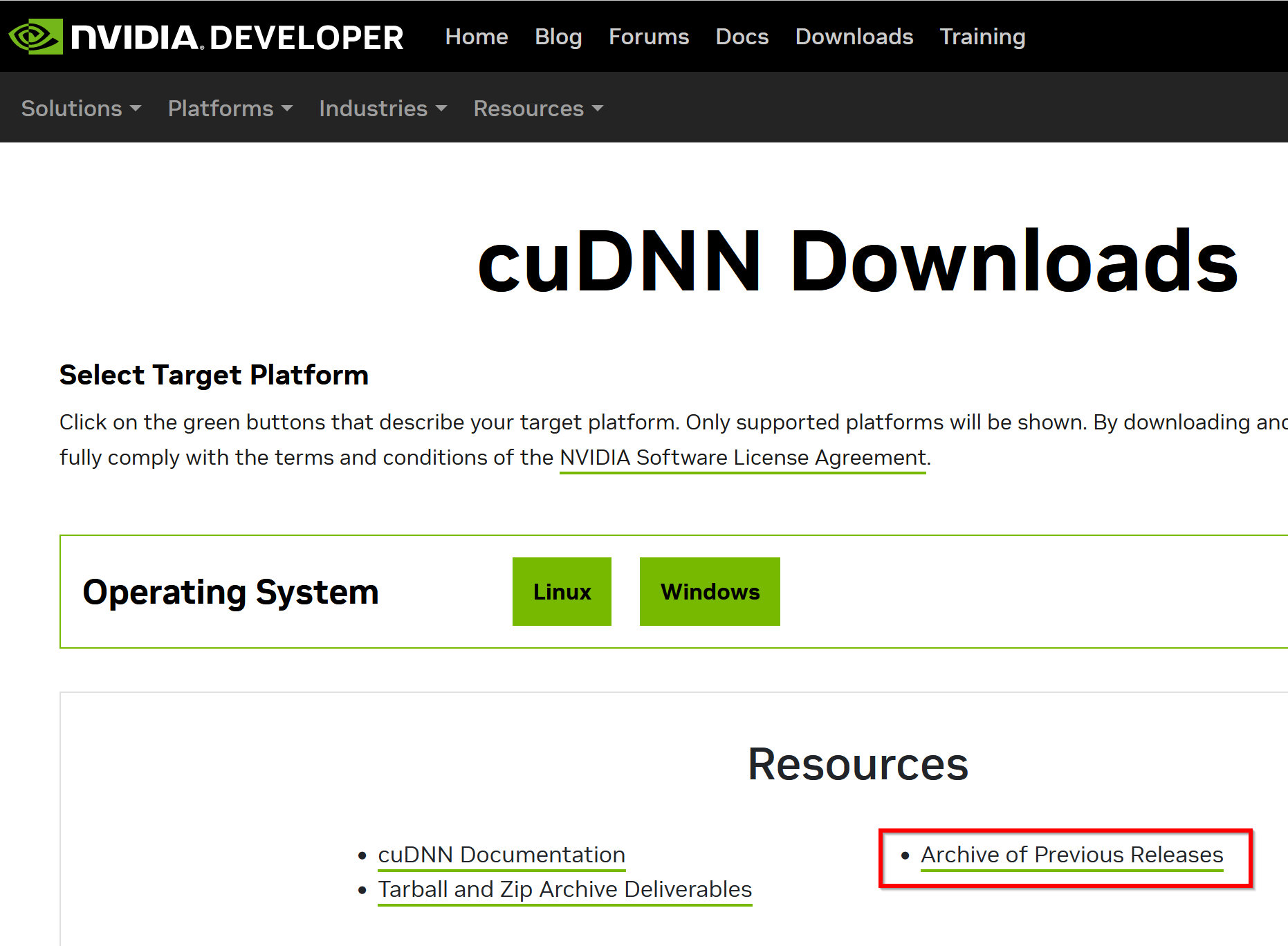
- NVIDIA cuDNN のウェブページを開く
- ダウンロードしたいので,cuDNNのところにある「Download cuDNN」をクリック.

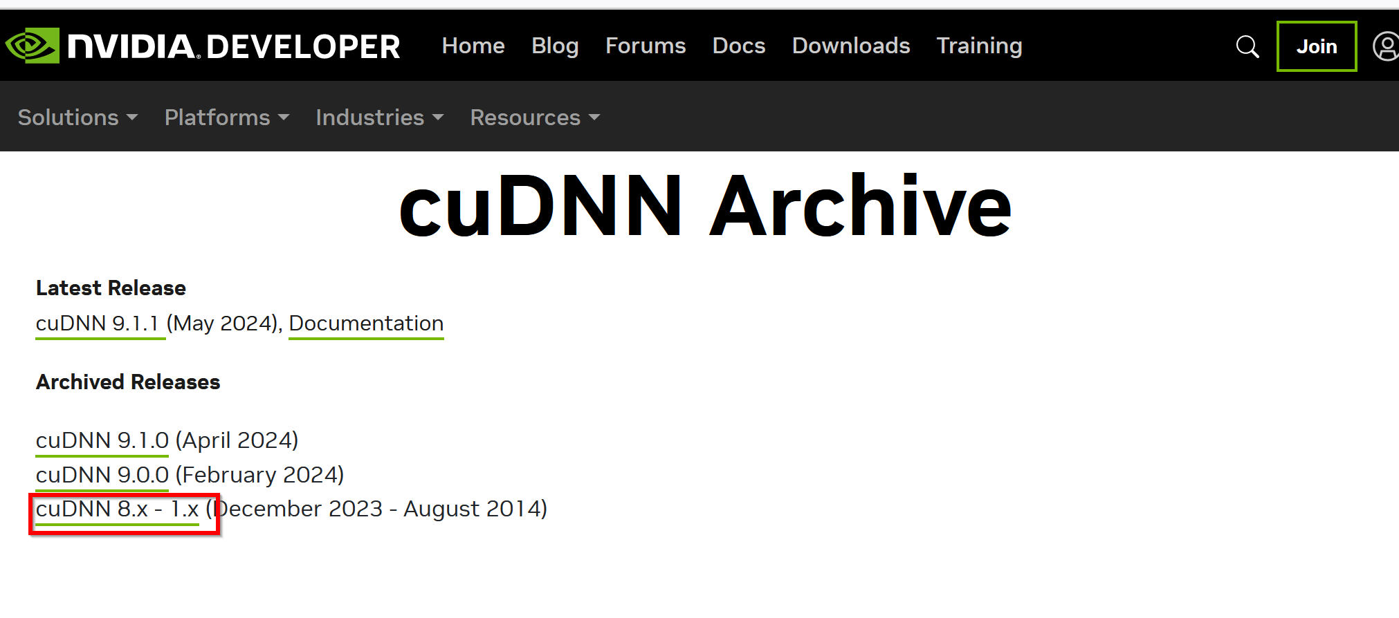
- cuDNN Downloads のページで「Archive of Previous Releases」をクリック
- 「cuDNN 8.x - 1.x」をクリック
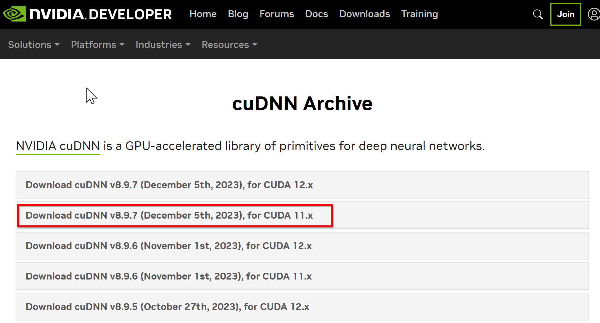
- ダウンロードしたいバージョンを選ぶ
ここでは「NVIDIA cuDNN v8.9.7 for CUDA 11.x」を選んでいる.
このとき,画面の「for CUDA ...」のところを確認し,使用するNVIDIA CUDA のバージョンに合うものを選ぶこと.
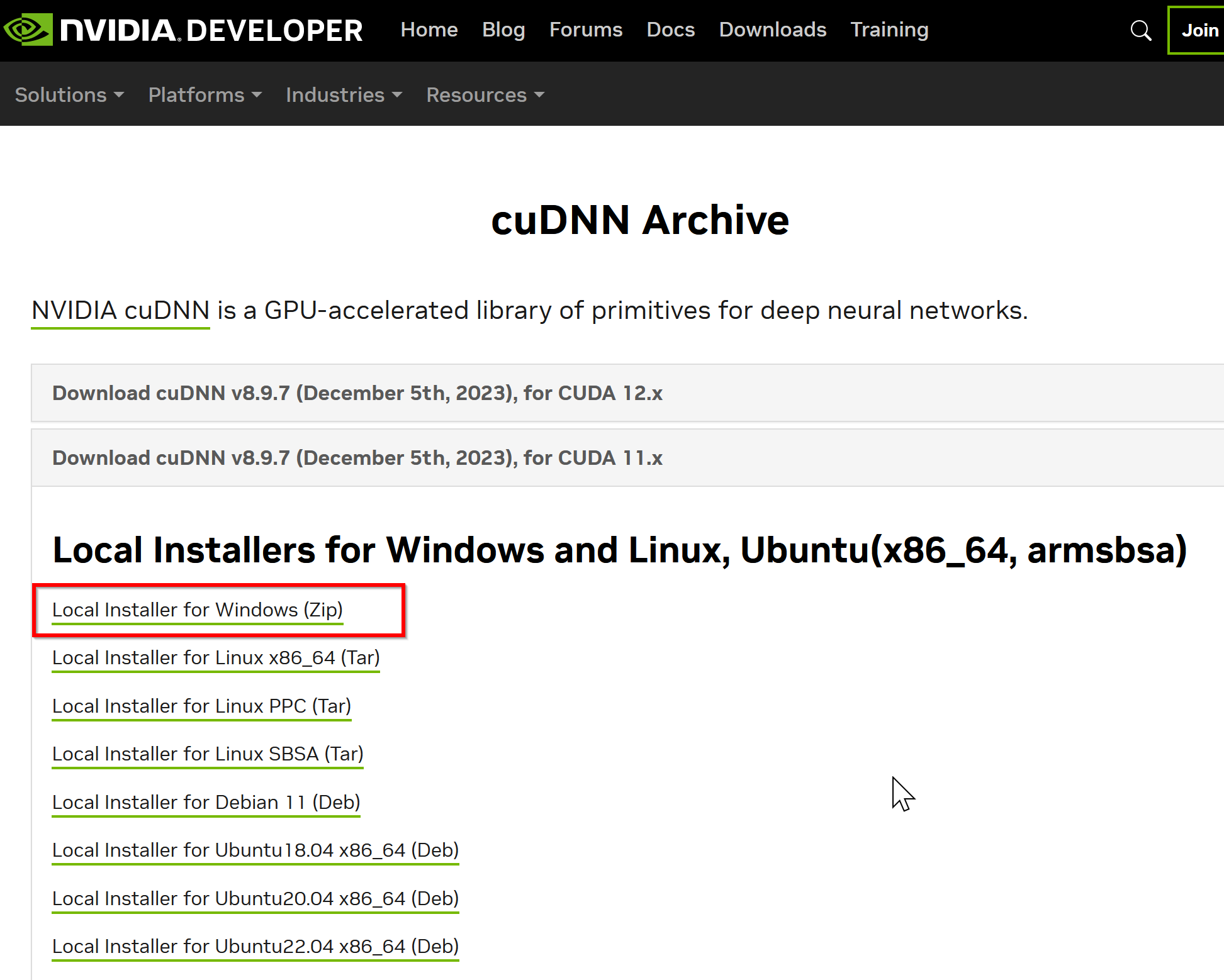
- Windows にインストールするので Windows 版を選ぶ
- NVIDIA Developer Program メンバーシップに入る
NVIDIA cuDNN のダウンロードのため.
「Join now」をクリック.その後,画面の指示に従う. 利用者本人が,電子メールアドレス,表示名,パスワード,生年月日を登録.利用条件等に合意.

- ログインする

- 調査の画面が出たときは,調査に応じる
- ライセンス条項の確認

- ダウンロードが始まる.
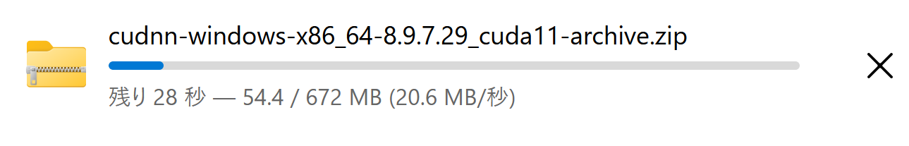
- ダウンロードした .zip ファイルを展開(解凍)する.
その中のサブディレクトリを確認しておく.
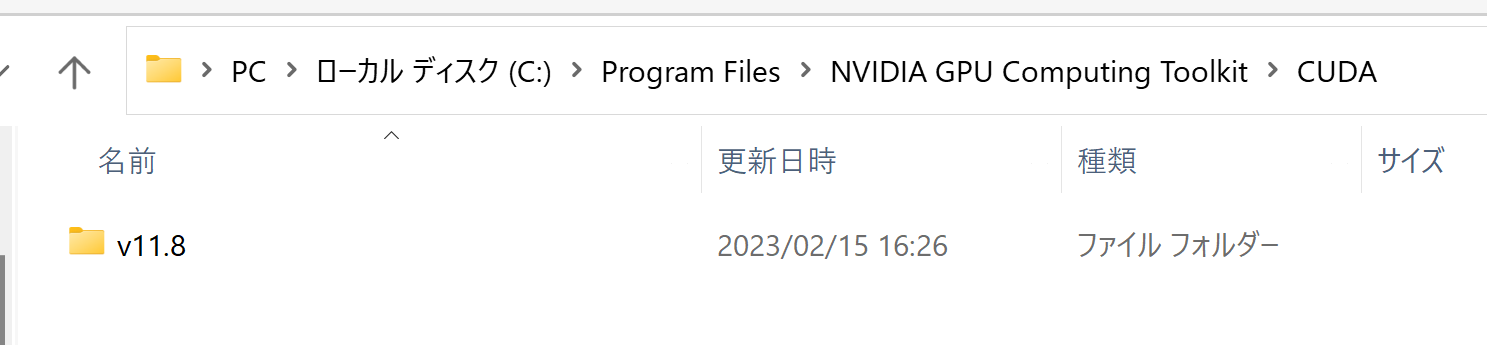
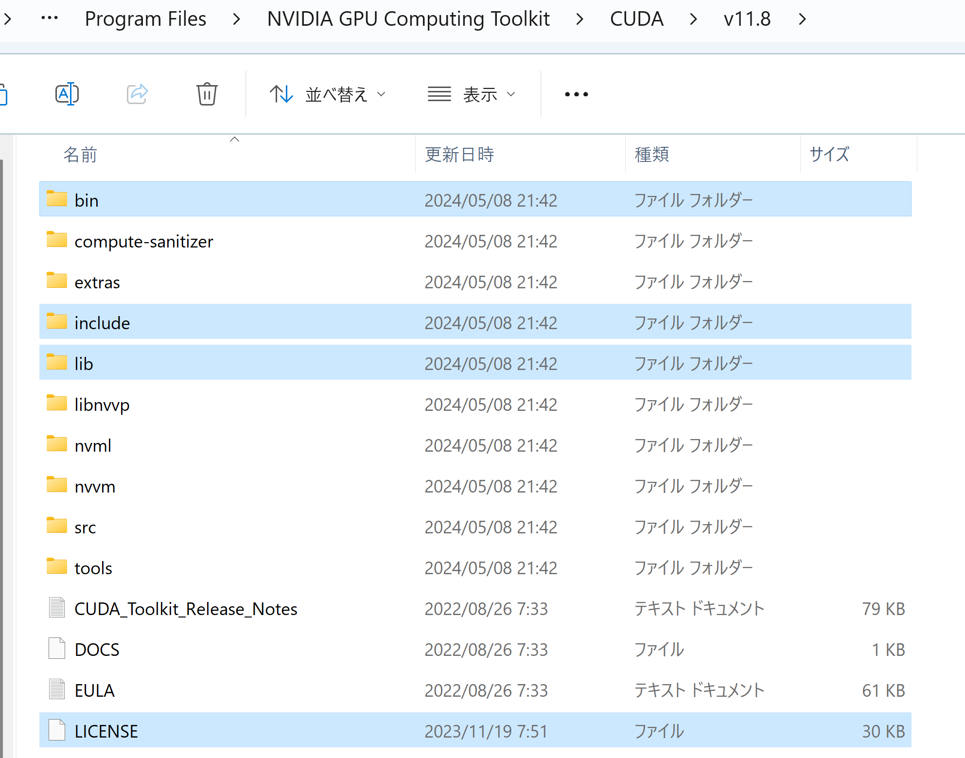
- NVIDIA CUDA ツールキットをインストールしたディレクトリを確認する.「C:\Program Files\NVIDIA GPU Computing Toolkit\CUDA\v11.8」のようになっている.
- 確認したら,
さきほど展開してできたすべてのファイルとディレクトリを,NVIDIA CUDA ツールキットをインストールしたディレクトリにコピーする
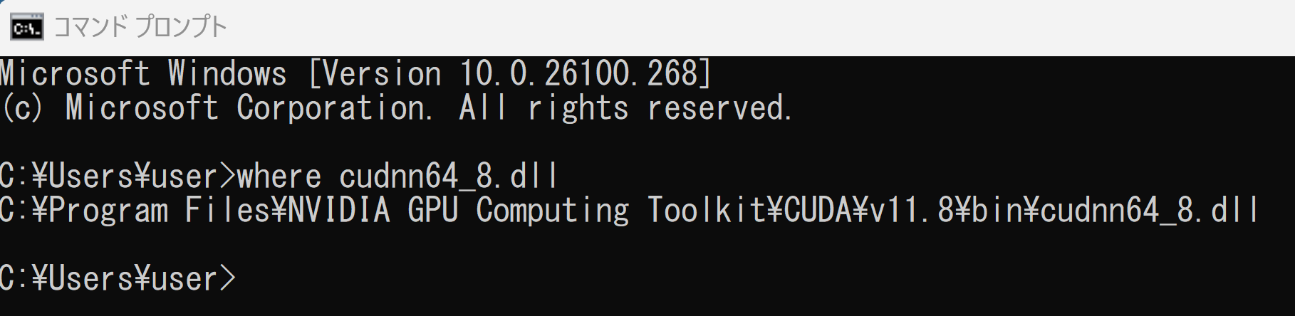
- パスが通っていることを確認.
次の操作により,cudnn64_8.dll にパスが通っていることを確認する.
Windows のコマンドプロンプトを開き,次のコマンドを実行する.エラーメッセージが出ないことを確認.
where cudnn64_8.dll
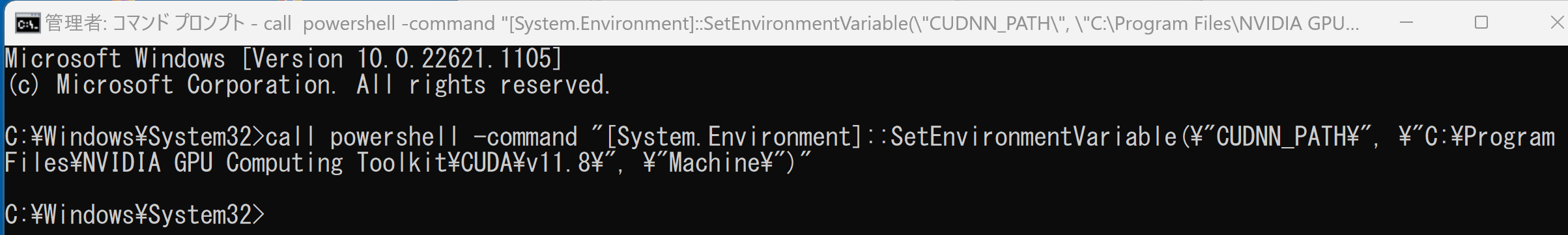
- Windows の システム環境変数 CUDNN_PATH の設定を行う.
Windows では,
コマンドプロンプトを管理者として開き,
次のコマンドを実行することにより,
システム環境変数 CUDNN_PATH の設定を行うことができる.
コマンドプロンプトを管理者として実行: 別ページ »で説明
powershell -command "[System.Environment]::SetEnvironmentVariable(\"CUDNN_PATH\", \"C:\Program Files\NVIDIA GPU Computing Toolkit\CUDA\v11.8\", \"Machine\")"
- Windows で,管理者権限でコマンドプロンプトを起動(手順:Windowsキーまたはスタートメニュー >
cmdと入力 > 右クリック > 「管理者として実行」)。 - TensorFlow 2.10.1 のインストール(Windows 上)
次のコマンドを実行することにより,TensorFlow 2.10.1 および関連パッケージ(tf_slim,tensorflow_datasets,tensorflow-hub,Keras,keras-tuner,keras-visualizer)がインストール(インストール済みのときは最新版に更新)される. そして,Pythonパッケージ(Pillow, pydot, matplotlib, seaborn, pandas, scipy, scikit-learn, scikit-learn-intelex, opencv-python, opencv-contrib-python)がインストール(インストール済みのときは最新版に更新)される.
python -m pip uninstall -y protobuf tensorflow tensorflow-cpu tensorflow-gpu tensorflow-intel tensorflow-text tensorflow-estimator tf-models-official tf_slim tensorflow_datasets tensorflow-hub keras keras-tuner keras-visualizer
python -m pip install -U protobuf tensorflow==2.10.1 tf_slim tensorflow_datasets==4.8.3 tensorflow-hub tf-keras keras keras_cv keras-tuner keras-visualizer
python -m pip install git+https://github.com/tensorflow/docs
python -m pip install git+https://github.com/tensorflow/examples.git
python -m pip install git+https://www.github.com/keras-team/keras-contrib.git
python -m pip install -U pillow pydot matplotlib seaborn pandas scipy scikit-learn scikit-learn-intelex opencv-python opencv-contrib-python
- Windows で,管理者権限でコマンドプロンプトを起動(手順:Windowsキーまたはスタートメニュー >
cmdと入力 > 右クリック > 「管理者として実行」)。次のコマンドを実行する.
python -m pip install -U numpy matplotlib seaborn scikit-learn pandas pydot
- Windows で,コマンドプロンプトを実行.
- jupyter qtconsole の起動
これ以降の操作は,jupyter qtconsole で行う.
jupyter qtconsole
Python 開発環境として,Jupyter Qt Console, Jupyter ノートブック (Jupyter Notebook), Jupyter Lab, Nteract, spyder のインストール
Windows で,管理者権限でコマンドプロンプトを起動(手順:Windowsキーまたはスタートメニュー >
cmdと入力 > 右クリック > 「管理者として実行」)。し,次のコマンドを実行する.次のコマンドを実行することにより,pipとsetuptoolsを更新する,Jupyter Notebook,PyQt5、Spyderなどの主要なPython環境がインストールされる.
python -m pip install -U pip setuptools requests notebook==6.5.7 jupyterlab jupyter jupyter-console jupytext PyQt5 nteract_on_jupyter spyder
- パッケージのインポート,TensorFlow のバージョン確認など
from __future__ import absolute_import, division, print_function, unicode_literals
import tensorflow as tf
from tensorflow.keras import layers
from tensorflow.keras import backend as K
K.clear_session()
import numpy as np
import tensorflow_datasets as tfds
from tensorflow.keras.preprocessing import image

%matplotlib inline
import matplotlib.pyplot as plt
import warnings
warnings.filterwarnings('ignore')   # Suppress Matplotlib warnings

# TensorFlow のバージョン
print(tf.__version__)

# GPU を利用しているか
gpus = tf.config.list_physical_devices(device_type = 'GPU')
if len(gpus)>0:
    print(f">> GPU detected. {gpus[0].name}")
    tf.config.experimental.set_memory_growth(gpus[0], True)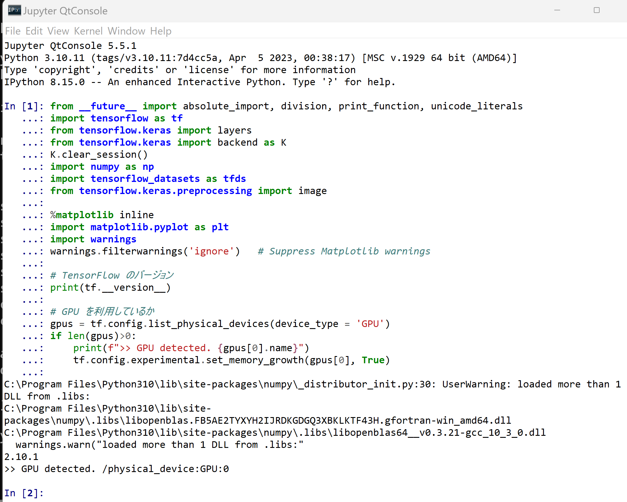
- MNIST データセットのロード
mnist, mnist_info = tfds.load('mnist', with_info = True, shuffle_files=True, as_supervised=True)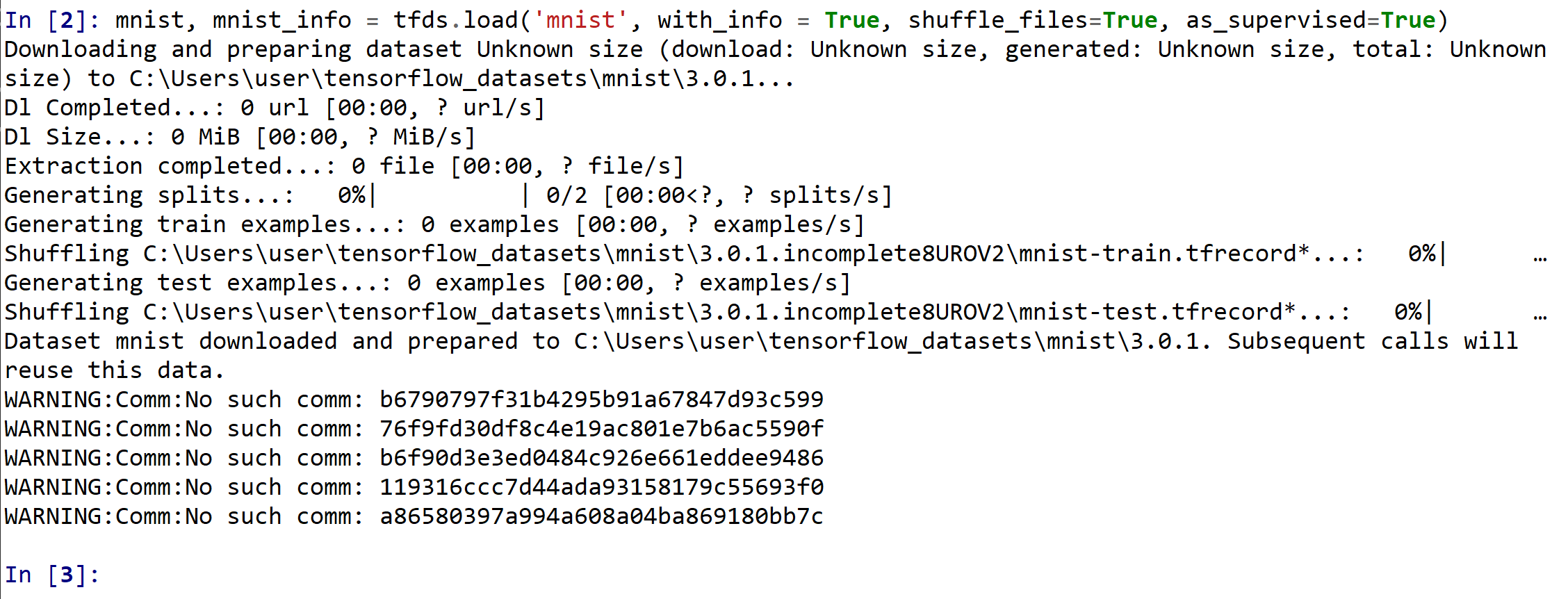
MNIST データセットの確認
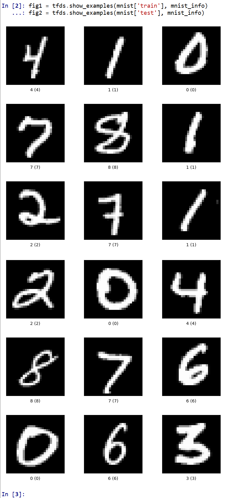
- データセットの中の画像を表示
fig1 = tfds.show_examples(mnist['train'], mnist_info)
fig2 = tfds.show_examples(mnist['test'], mnist_info)
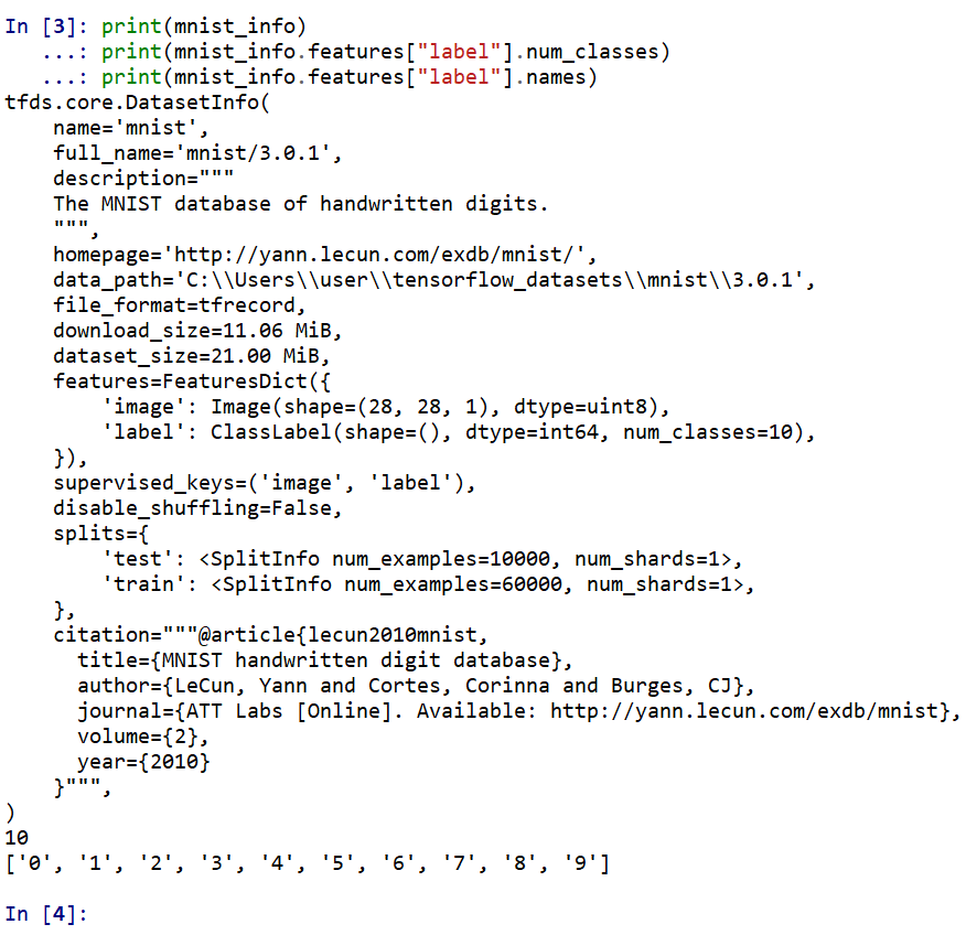
- データセットの情報を表示
print(mnist_info)
print(mnist_info.features["label"].num_classes)
print(mnist_info.features["label"].names)
Keras を用いたニューラルネットワークの作成
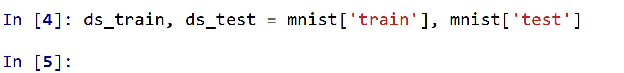
- データセットの生成
ds_train: サイズ 28 × 28 の 60000枚の濃淡画像,60000枚の濃淡画像それぞれのラベル(0 から 9 のどれか)
ds_test: サイズ 28 × 28 の 60000枚の濃淡画像,60000枚の濃淡画像それぞれのラベル(0 から 9 のどれか)
ds_train, ds_test = mnist['train'], mnist['test']
- 確認のため,データセットの先頭要素を確認してみる
次により,データセット ds_train, ds_test の先頭要素を確認.
次のプログラムでは,ds_train, ds_test の先頭要素が,i に得られる. i がタップルであること, そして,i は TensorFlow のテンソルが並んだタップルであることを確認する.
実行結果からは,次を確認,i の長さは 2,そして,i の中身が 2つであることが分かる.
- ds_train の先頭要素: 形状 (28, 28, 1) と形状 () のタップル
- ds_test の先頭要素: 形状 (28, 28, 1) と形状 () のタップル
for i in ds_train.take(1):
    print(type(i))
    for j in range(len(i)):
        print(type(i[j]))
        print(i[j].shape)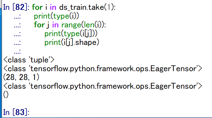
for i in ds_test.take(1):
    print(type(i))
    for j in range(len(i)):
        print(type(i[j]))
        print(i[j].shape)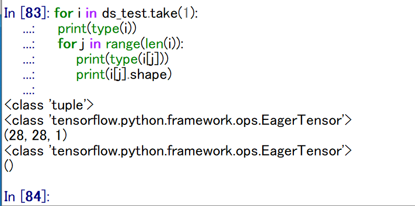
- 確認のため,データセットの先頭要素を表示してみる
「tf.reshape(image, [-1])」では,テンソルをフラット化している.これは,表示を見やすくするため.
タップルの 0 番目は数値データ, タップルの 1 番目は分類結果のラベル(クラス名)である.
for image, label in ds_train.take(1):
    print(tf.reshape(image, [-1]))
    print(label)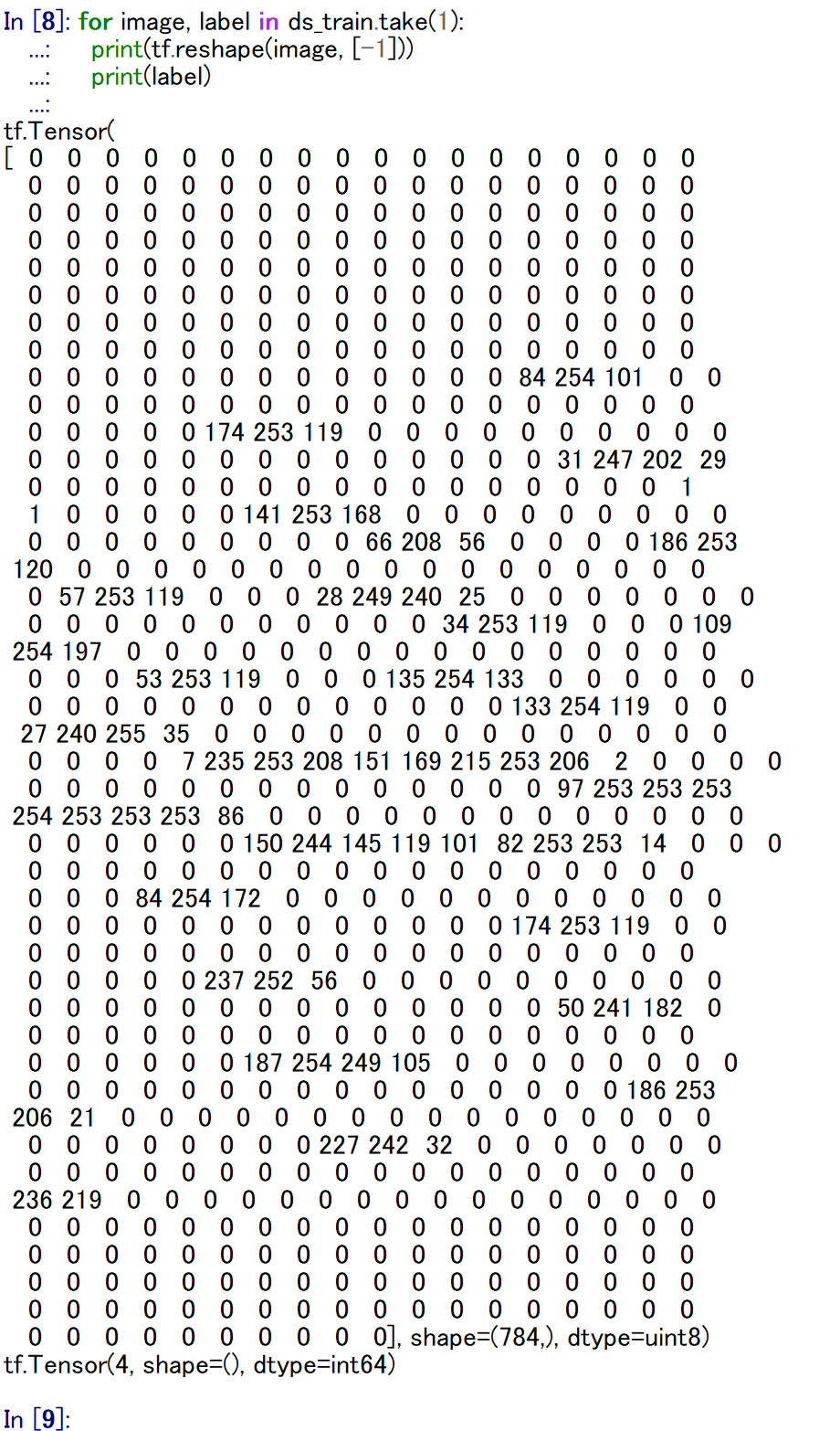
for image, label in ds_test.take(1):
    print(tf.reshape(image, [-1]))
    print(label)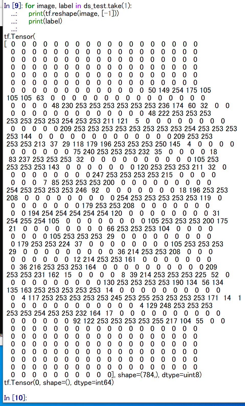
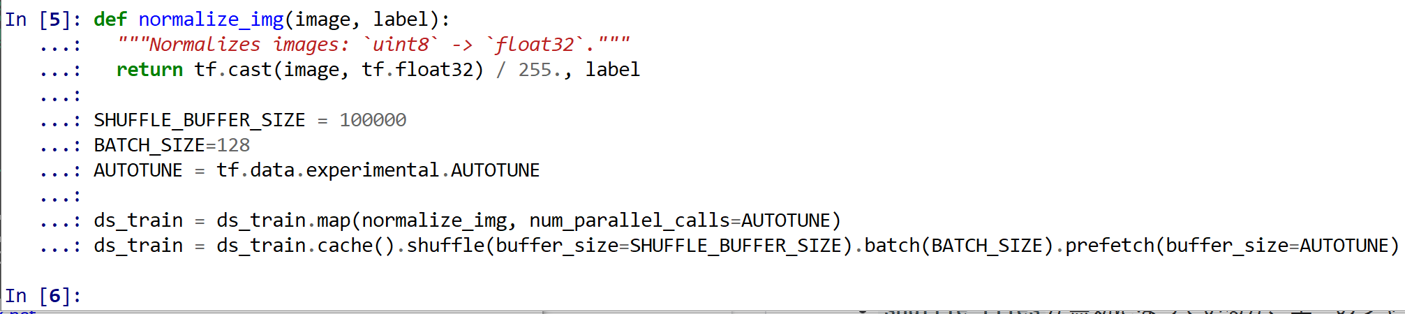
- トレーニングパイプライン
値は,もともと int で 0 から 255 の範囲であるのを, float32 で 0 から 1 の範囲になるように前処理を行う.そして, データセットのシャッフルとバッチも行う.
def normalize_img(image, label):
  """Normalizes images: `uint8` -> `float32`."""
  return tf.cast(image, tf.float32) / 255., label

SHUFFLE_BUFFER_SIZE = 100000
BATCH_SIZE=128
AUTOTUNE = tf.data.experimental.AUTOTUNE

ds_train = ds_train.map(normalize_img, num_parallel_calls=AUTOTUNE)
ds_train = ds_train.cache().shuffle(buffer_size=SHUFFLE_BUFFER_SIZE).batch(BATCH_SIZE).prefetch(buffer_size=AUTOTUNE)
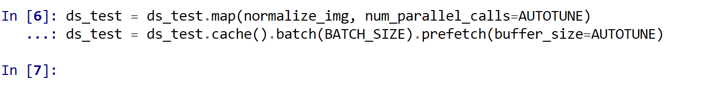
- 評価パイプライン
値は,もともと int で 0 から 255 の範囲であるのを, float32 で 0 から 1 の範囲になるように前処理を行う.そして, データセットのバッチも行う.
ds_test = ds_test.map(normalize_img, num_parallel_calls=AUTOTUNE)
ds_test = ds_test.cache().batch(BATCH_SIZE).prefetch(buffer_size=AUTOTUNE)
- モデルの作成と確認
num_classes = 10
input_shape = (28, 28)
m = tf.keras.Sequential(
    [
        tf.keras.Input(shape=input_shape),
        layers.Flatten(),
        layers.Dense(units=64, activation='relu'),
        layers.Dropout(0.5),
        layers.Dense(units=num_classes, activation='softmax')
    ]
)
print(m.summary())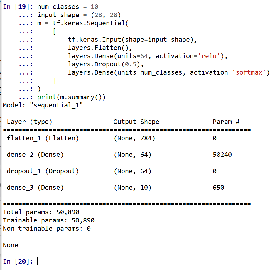
L2 正則化を行いたいときは 「 tf.keras.layers.Dense(64, activation='relu', kernel_regularizer=tf.keras.regularizers.l2(0.001)),」のようにする.
ニューラルネットワークの学習と検証
- コンパイル,学習を行う
ニューラルネットワークの学習は fit メソッドにより行う. 教師データを使用する. 教師データを投入する.
EPOCHS = 20
m.compile(
    optimizer=tf.keras.optimizers.Adam(learning_rate=0.001),
    loss='sparse_categorical_crossentropy',
    metrics=['sparse_categorical_crossentropy', 'accuracy']
)
history = m.fit(ds_train,
                    batch_size=128,
                    epochs=EPOCHS,
                    validation_data=ds_test,
                    verbose=1)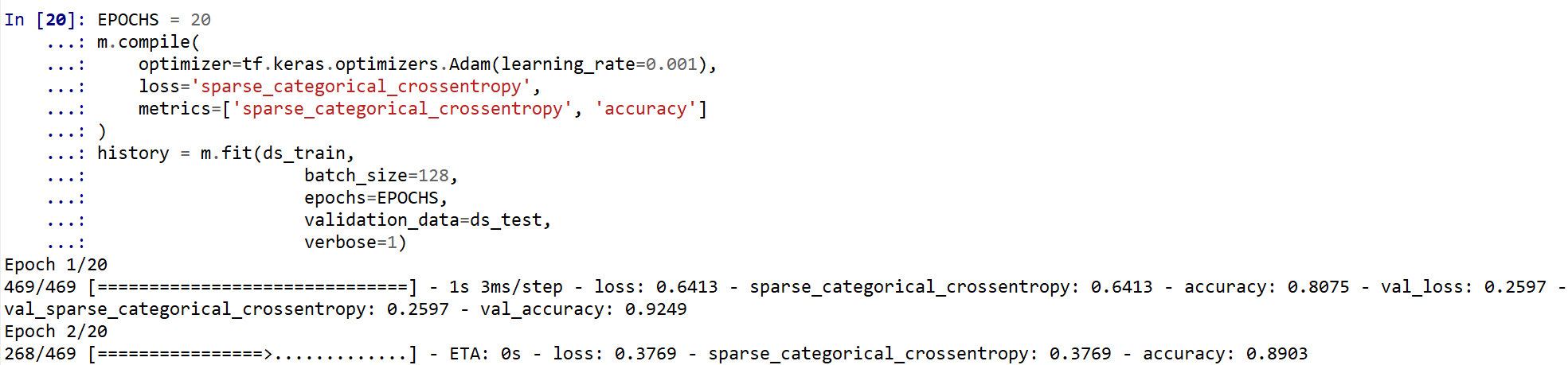
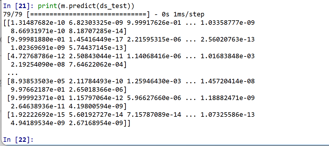
(以下省略) - ディープラーニングによるデータの分類
ds_test を分類してみる.
print(m.predict(ds_test))
それぞれの数値の中で、一番大きいものはどれか?
m.predict(ds_test).argmax(axis=1)
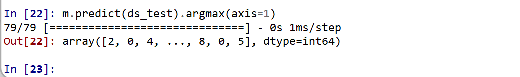
ds_test 内にある正解のラベル(クラス名)を表示する(上の結果と比べるため)
for i in ds_test:
    print(i[1])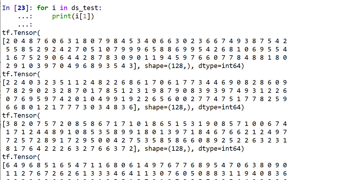
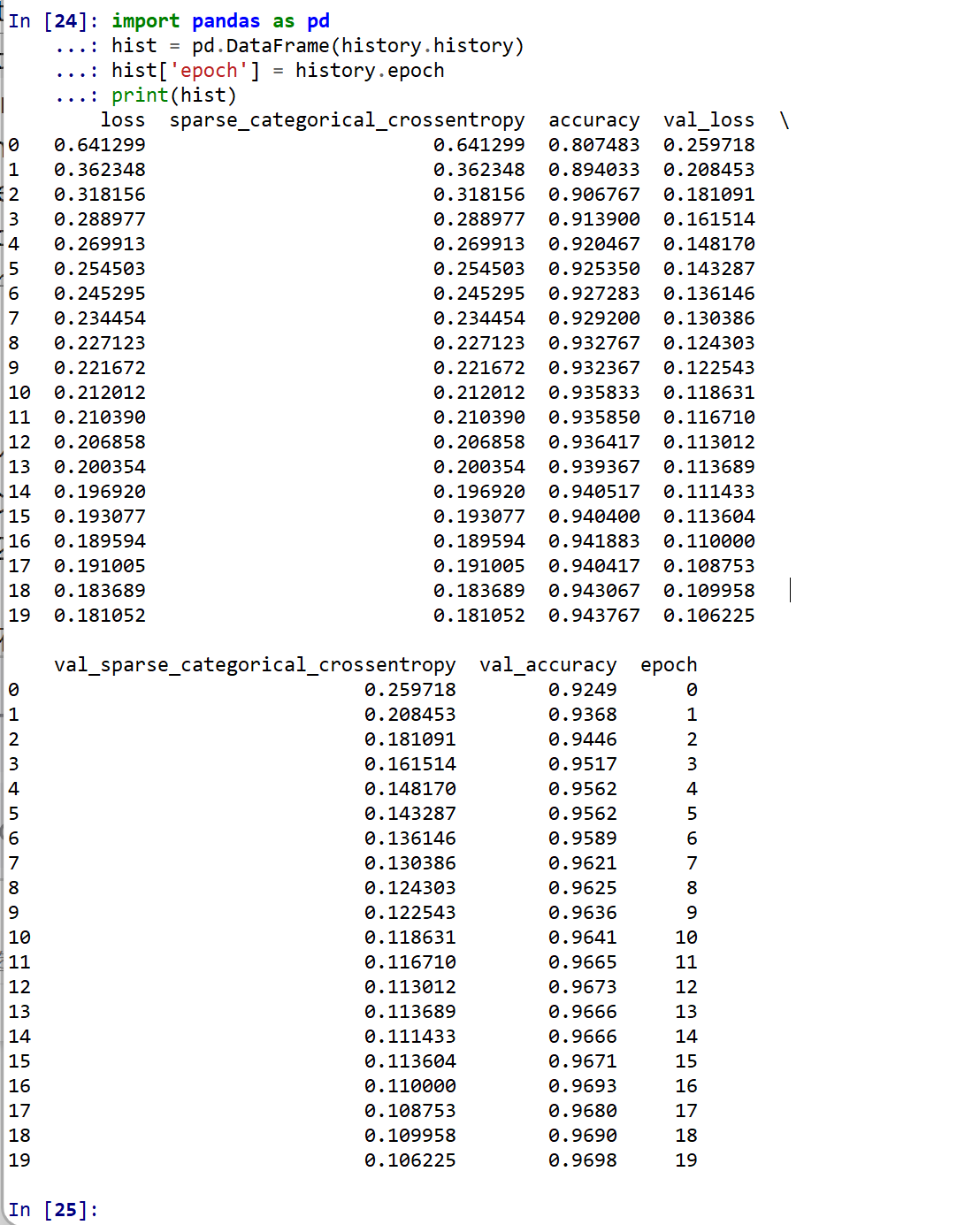
- 学習曲線の確認
過学習や学習不足について確認.
import pandas as pd
hist = pd.DataFrame(history.history)
hist['epoch'] = history.epoch
print(hist)
【関連する外部ページ】 訓練の履歴の可視化については,https://keras.io/ja/visualization/
- 学習時と検証時の,損失の違い
acc = history.history['accuracy']
val_acc = history.history['val_accuracy']
loss = history.history['loss']
val_loss = history.history['val_loss']

epochs = range(1, len(acc) + 1)

# "bo" は青いドット
plt.plot(epochs, loss, 'bo', label='Training loss')
# ”b" は青い実線
plt.plot(epochs, val_loss, 'b', label='Validation loss')
plt.title('Training and validation loss')
plt.xlabel('Epochs')
plt.ylabel('Loss')
plt.legend()

plt.show()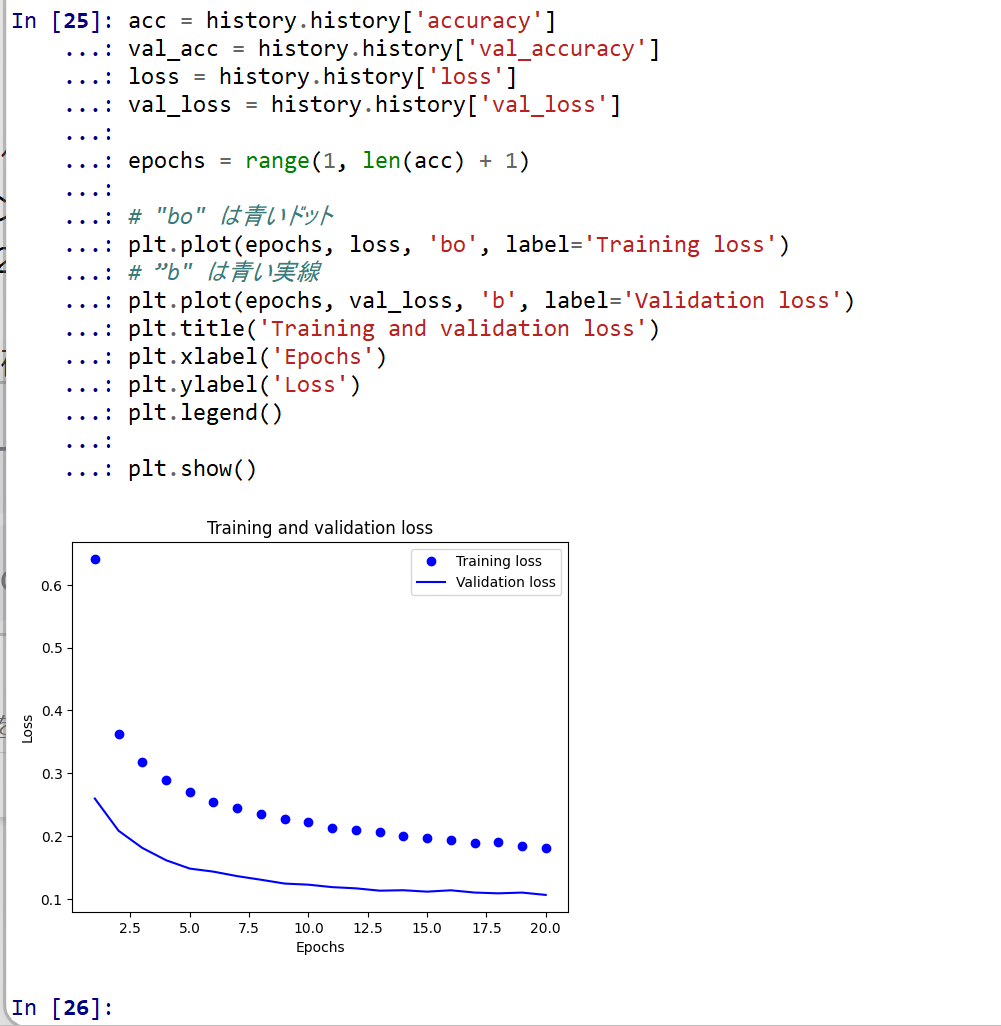
- 学習時と検証時の,精度の違い
acc = history.history['accuracy']
val_acc = history.history['val_accuracy']
loss = history.history['loss']
val_loss = history.history['val_loss']

plt.clf()   # 図のクリア
plt.plot(epochs, acc, 'bo', label='Training acc')
plt.plot(epochs, val_acc, 'b', label='Validation acc')
plt.title('Training and validation accuracy')
plt.xlabel('Epochs')
plt.ylabel('Accuracy')
plt.legend()

plt.show()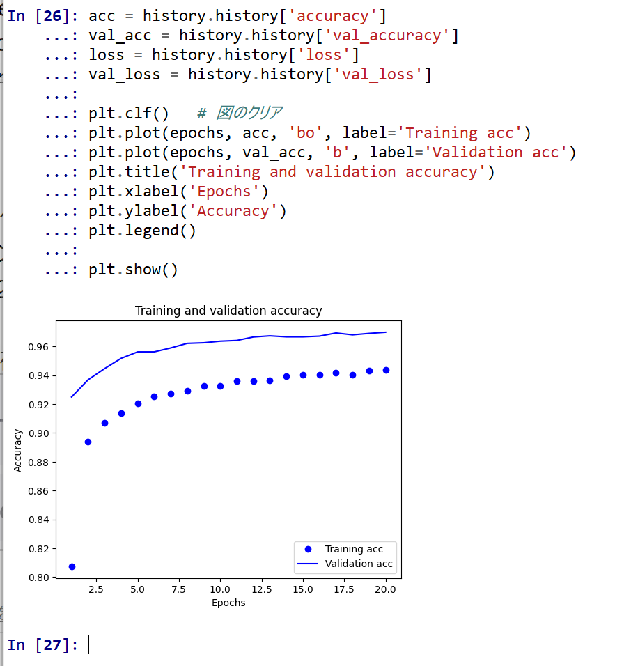
- 学習時と検証時の,損失の違い
- パッケージのインポート,TensorFlow のバージョン確認など
NVIDIA CUDA ツールキット 11.8 のインストール(Windows 上)
CUDAツールキットには、GPUでプログラムを実行するためのライブラリ、`nvcc`コンパイラ、開発ツールなどが含まれています。ここでは`winget`を使ってCUDA 11.8をインストールする手順を示します。
NVIDIA CUDA ツールキットの概要と注意点
NVIDIAのGPUを使用して並列計算を行うための開発・実行環境です。
主な機能: GPU を利用した並列処理のコンパイルと実行、GPU のメモリ管理、C++をベースとした拡張言語(CUDA C/C++)とAPI、ライブラリ(cuBLAS, cuFFTなど)を提供します。
【NVIDIA CUDA ツールキットの動作に必要なもの】
【Windows でインストールするときの一般的な注意点】
【関連する外部ページ】
【関連項目】 NVIDIA CUDA ツールキットの概要, NVIDIA CUDA ツールキットの他バージョンのインストール
NVIDIA cuDNN 8.9.7 のインストール(Windows 上)
NVIDIA cuDNN
NVIDIA cuDNN は,NVIDIA CUDA ツールキット上で動作する、高性能なディープラーニング用ライブラリです.畳み込みニューラルネットワーク (CNN) やリカレントニューラルネットワーク (RNN) など,さまざまなディープラーニングモデルのトレーニングと推論を高速化します.
【cuDNN利用時の注意点: zlibwapi.dll エラー】
Windows環境でcuDNNを利用するアプリケーションを実行した際に、「Could not locate zlibwapi.dll. Please make sure it is in your library path!」というエラーが表示されることがあります。これは、cuDNNの一部の機能が圧縮ライブラリである zlib に依存しているためです。このエラーが発生した場合は、後述する手順で ZLIB DLL をインストールする必要があります。
【関連する外部ページ】
NVIDIA cuDNN のインストール(Windows 上)の概要
zlib のインストール(Windows 上)
【関連する外部ページ】
【関連項目】 zlib
NVIDIA cuDNN 8.9.7 のインストール(Windows 上)
TensorFlow 2.10.1 のインストール(Windows 上)
Graphviz のインストール
Windows での Graphviz のインストール: 別ページ »で説明
numpy,matplotlib, seaborn, scikit-learn, pandas, pydot のインストール
MNIST データセットのロード
【Python の利用】
Python は,次のコマンドで起動できる.
Python 開発環境(Jupyter Qt Console, Jupyter ノートブック (Jupyter Notebook), Jupyter Lab, Nteract, Spyder, PyCharm, PyScripterなど)も便利である.
Python のまとめ: 別ページ »にまとめ