CNN による画像分類,モデルの作成と学習と検証(MobileNetV2,ResNet50,DenseNet 121,DenseNet 169,NASNet,TensorFlow データセットのCIFAR-10 データセットを使用)(Google Colab 上もしくはパソコン上)
CNN の作成,学習,画像分類を行う. TensorFlow データセットのCIFAR-10 データセットを使用する. CNN としては,次のものを使用する.
【目次】
- Google Colaboratory での実行
- Windows での実行
- CIFAR-10 データセットのロード
- CIFAR-10 データセットの確認
- ニューラルネットワークの作成(MobileNetV2 を使用)
- ニューラルネットワークの作成(ResNet50 を使用)
- ニューラルネットワークの作成(DenseNet 121 を使用)
- ニューラルネットワークの作成(DenseNet 169 を使用)
- ニューラルネットワークの作成(NASNet を使用)
【サイト内の関連ページ】
- CNN による画像分類: https://www.kkaneko.jp/ai/imclassify/index.html
- 関連の用語集: https://www.kkaneko.jp/tools/man/man.html
【関連する外部ページ】
- Keras の応用のページ: https://keras.io/ja/applications/
1. Google Colaboratory での実行
Google Colaboratory のページ:
https://colab.research.google.com/drive/1fNGbsjqt2FgO_QGoW0n74CQR77iAX2li?usp=sharing
2. Windows での実行
Python 3.12 のインストール(Windows 上) [クリックして展開]
以下のいずれかの方法で Python 3.12 をインストールする。Python がインストール済みの場合、この手順は不要である。
方法1:winget によるインストール
管理者権限のコマンドプロンプトで以下を実行する。管理者権限のコマンドプロンプトを起動するには、Windows キーまたはスタートメニューから「cmd」と入力し、表示された「コマンドプロンプト」を右クリックして「管理者として実行」を選択する。
winget install --id Python.Python.3.12 -e --scope machine --silent --accept-source-agreements --accept-package-agreements --override "/quiet InstallAllUsers=1 PrependPath=1 Include_test=0 Include_pip=1 Include_launcher=1 InstallLauncherAllUsers=1 TargetDir=\"C:\Program Files\Python312\""
powershell -Command "$p='C:\Program Files\Python312'; $s=\"$p\Scripts\"; $m=[Environment]::GetEnvironmentVariable('Path','Machine'); if($m -notlike \"*$s*\") { [Environment]::SetEnvironmentVariable('Path', \"$p;$s;$m\", 'Machine') }"
--scope machine を指定することで、システム全体(全ユーザー向け)にインストールされる。このオプションの実行には管理者権限が必要である。インストール完了後、コマンドプロンプトを再起動すると PATH が自動的に設定される。
方法2:インストーラーによるインストール
- Python 公式サイト(https://www.python.org/downloads/)にアクセスし、「Download Python 3.x.x」ボタンから Windows 用インストーラーをダウンロードする。
- ダウンロードしたインストーラーを実行する。
- 初期画面の下部に表示される「Add python.exe to PATH」に必ずチェックを入れてから「Customize installation」を選択する。このチェックを入れ忘れると、コマンドプロンプトから
pythonコマンドを実行できない。 - 「Install Python 3.xx for all users」にチェックを入れ、「Install」をクリックする。
インストールの確認
コマンドプロンプトで以下を実行する。
python --versionバージョン番号(例:Python 3.12.x)が表示されればインストール成功である。「'python' は、内部コマンドまたは外部コマンドとして認識されていません。」と表示される場合は、インストールが正常に完了していない。
Git のインストール
管理者権限のコマンドプロンプトで以下を実行する。管理者権限のコマンドプロンプトを起動するには、Windows キーまたはスタートメニューから「cmd」と入力し、表示された「コマンドプロンプト」を右クリックして「管理者として実行」を選択する。
REM Git をシステム領域にインストール
winget install --scope machine --id Git.Git -e --silent --disable-interactivity --force --accept-source-agreements --accept-package-agreements --override "/VERYSILENT /NORESTART /NOCANCEL /SP- /CLOSEAPPLICATIONS /RESTARTAPPLICATIONS /COMPONENTS=""icons,ext\reg\shellhere,assoc,assoc_sh"" /o:PathOption=Cmd /o:CRLFOption=CRLFCommitAsIs /o:BashTerminalOption=MinTTY /o:DefaultBranchOption=main /o:EditorOption=VIM /o:SSHOption=OpenSSH /o:UseCredentialManager=Enabled /o:PerformanceTweaksFSCache=Enabled /o:EnableSymlinks=Disabled /o:EnableFSMonitor=Disabled"
【関連する外部ページ】
- Git の公式ページ: https://git-scm.com/
TensorFlow 2.10.1 のインストール(Windows 上)
- 以下の手順を管理者権限のコマンドプロンプトで実行する
(手順:Windowsキーまたはスタートメニュー →
cmdと入力 → 右クリック → 「管理者として実行」)。 - TensorFlow 2.10.1 のインストール(Windows 上)
次のコマンドを実行することにより,TensorFlow 2.10.1 および関連パッケージ(tf_slim,tensorflow_datasets,tensorflow-hub,Keras,keras-tuner,keras-visualizer)がインストール(インストール済みのときは最新版に更新)される. そして,Pythonライブラリ(Pillow, pydot, matplotlib, seaborn, pandas, scipy, scikit-learn, scikit-learn-intelex, opencv-python, opencv-contrib-python)がインストール(インストール済みのときは最新版に更新)される.
python -m pip uninstall -y protobuf tensorflow tensorflow-cpu tensorflow-gpu tensorflow-intel tensorflow-text tensorflow-estimator tf-models-official tf_slim tensorflow_datasets tensorflow-hub keras keras-tuner keras-visualizer
python -m pip install -U protobuf tensorflow==2.10.1 tf_slim tensorflow_datasets==4.8.3 tensorflow-hub tf-keras keras keras_cv keras-tuner keras-visualizer
python -m pip install git+https://github.com/tensorflow/docs
python -m pip install git+https://github.com/tensorflow/examples.git
python -m pip install git+https://www.github.com/keras-team/keras-contrib.git
python -m pip install -U pillow pydot matplotlib seaborn pandas scipy scikit-learn scikit-learn-intelex opencv-python opencv-contrib-python
Graphviz のインストール
Windows での Graphviz のインストール: 別ページ »で説明
numpy,matplotlib, seaborn, scikit-learn, pandas, pydot のインストール
- 次のコマンドを管理者権限のコマンドプロンプトで実行する
(手順:Windowsキーまたはスタートメニュー →
cmdと入力 → 右クリック → 「管理者として実行」)。 する.
python -m pip install -U numpy matplotlib seaborn scikit-learn pandas pydot
CIFAR-10 データセットのロード
Python 3.12 のインストール
Pythonのインストールを行い、Pythonのプログラムを実行する環境を整える。扱う環境は、Windows搭載パソコンである。金子研究室では、Python 3.12.10を推奨する。
[Windows での Python 3.12 のインストール手順を見るには、ここをクリック]
Windows での Python 3.12 のインストール
以下のいずれかの方法でPython 3.12をインストールする。Pythonがインストール済みの場合、この手順は不要である。
方法 1:winget によるインストール
【インストールコマンドの実行方法】
管理者権限でコマンドプロンプトを起動する(手順:Windowsキーまたはスタートメニュー → cmd と入力 → 右クリック → 「管理者として実行」)。そして、コマンド全体をコマンドプロンプトにコピー&ペーストする。
--scope machine を指定することで、システム全体(全ユーザー向け)にインストールされる。このオプションの実行には管理者権限が必要である。インストール完了後、コマンドプロンプトを再起動するとPATHが反映される。
REM Python 3.12 をシステム領域にインストール
winget install --id Python.Python.3.12 -e --scope machine --silent --accept-source-agreements --accept-package-agreements --override "/quiet InstallAllUsers=1 PrependPath=1 Include_test=0 Include_pip=1 Include_launcher=1 InstallLauncherAllUsers=1 TargetDir=\"C:\Program Files\Python312\""

REM Python と Scripts を PATH 先頭に追加
powershell -NoProfile -Command "$p='C:\Program Files\Python312'; $s=\"$p\Scripts\"; $c=[Environment]::GetEnvironmentVariable('Path','Machine'); if((Test-Path $p) -and (';'+$c+';' -notlike \"*;$p;*\") -and (';'+$c+';' -notlike \"*;$s;*\")){[Environment]::SetEnvironmentVariable('Path',\"$p;$s;$c\",'Machine')}"
方法 2:インストーラーによるインストール
- Python公式サイト(https://www.python.org/downloads/)にアクセスし、「Download Python 3.x.x」ボタンからWindows用インストーラーをダウンロードする。
- ダウンロードしたインストーラーを実行する。
- 初期画面の下部に表示される「Add python.exe to PATH」にチェックを入れてから「Customize installation」を選択する。このチェックを入れ忘れると、コマンドプロンプトから
pythonコマンドを実行できない。 - 「Install Python 3.xx for all users」にチェックを入れ、「Install」をクリックする。
インストールの確認
コマンドプロンプトで以下を実行する。
python --versionバージョン番号(例:Python 3.12.x)が表示されればインストール成功である。「'python' は、内部コマンドまたは外部コマンドとして認識されていません。」と表示される場合は、インストールが正常に完了していない。
Python の開発環境 Visual Studio Code のインストールと Python 用の設定
Python の開発環境Visual Studio Code(プログラムを編集するソフトウェア。以下、VS Code)を整える。
[Windows での Visual Studio Code のインストールと Python 用の設定手順を見るには、ここをクリック]
Windows での Visual Studio Code のインストールと Python 用の設定手順
1. VS Code と拡張機能のインストール
以下のコマンドにより,既存の VS Code を削除し,全ユーザー共有の設定で再インストールしたうえで,拡張機能(VS Code に機能を追加するソフトウェア)をまとめて導入する.
【インストールコマンドの実行方法】
管理者権限でコマンドプロンプトを起動する(手順:Windows キーまたはスタートメニュー → cmd と入力 → 右クリック → 「管理者として実行」)。そして,コマンド全体をコマンドプロンプトにコピー&ペーストする。
インストールコマンド
REM ============================================================
REM Microsoft Visual Studio Code
REM ============================================================
winget uninstall -e --id Microsoft.VisualStudioCode --silent --disable-interactivity --accept-source-agreements
rmdir /s /q C:\ProgramData\vscode-extensions 2>nul
rmdir /s /q "%APPDATA%\Code" 2>nul
rmdir /s /q "%USERPROFILE%\.vscode" 2>nul
rmdir /s /q "%LOCALAPPDATA%\Microsoft\vscode-update" 2>nul

REM VS Code をシステム領域に新規インストール
winget install --scope machine --id Microsoft.VisualStudioCode -e --silent --accept-source-agreements --accept-package-agreements

REM 全ユーザー共有の拡張機能フォルダ
mkdir C:\ProgramData\vscode-extensions 2>nul
icacls "C:\ProgramData\vscode-extensions" /grant "Everyone:(OI)(CI)M" /T

REM スタートメニューのショートカットを --extensions-dir 付きで再作成
rmdir /s /q "C:\ProgramData\Microsoft\Windows\Start Menu\Programs\Visual Studio Code" 2>nul
del "C:\ProgramData\Microsoft\Windows\Start Menu\Programs\Visual Studio Code.lnk" 2>nul
powershell -NoProfile -Command "$s=New-Object -ComObject WScript.Shell; $lnk=$s.CreateShortcut('C:\ProgramData\Microsoft\Windows\Start Menu\Programs\Visual Studio Code.lnk'); $lnk.TargetPath='C:\Program Files\Microsoft VS Code\Code.exe'; $lnk.Arguments='--extensions-dir \"C:\ProgramData\vscode-extensions\"'; $lnk.Save()"
REM ショートカットの検証
powershell -NoProfile -Command "$s=New-Object -ComObject WScript.Shell; $lnk=$s.CreateShortcut('C:\ProgramData\Microsoft\Windows\Start Menu\Programs\Visual Studio Code.lnk'); Write-Host 'TargetPath:' $lnk.TargetPath; Write-Host 'Arguments:' $lnk.Arguments"

REM ファイル / フォルダ右クリックの「Code で開く」を登録
reg add "HKLM\SOFTWARE\Classes\*\shell\VSCode\command" /ve /d "\"C:\Program Files\Microsoft VS Code\Code.exe\" --extensions-dir \"C:\ProgramData\vscode-extensions\" \"%1\"" /f
reg add "HKLM\SOFTWARE\Classes\Directory\shell\VSCode\command" /ve /d "\"C:\Program Files\Microsoft VS Code\Code.exe\" --extensions-dir \"C:\ProgramData\vscode-extensions\" \"%1\"" /f
reg add "HKLM\SOFTWARE\Classes\Directory\Background\shell\VSCode\command" /ve /d "\"C:\Program Files\Microsoft VS Code\Code.exe\" --extensions-dir \"C:\ProgramData\vscode-extensions\" \"%V\"" /f

REM --extensions-dir 付きで起動する code.cmd ラッパを作成
REM (%* を echo で書くと対話的 cmd で失われるため、PowerShell で [char]37+'*' を書き出す)
powershell -NoProfile -Command "$pct=[char]37; $q=[char]34; $c='@echo off'+[char]13+[char]10+$q+'C:\Program Files\Microsoft VS Code\bin\code.cmd'+$q+' --extensions-dir '+$q+'C:\ProgramData\vscode-extensions'+$q+' '+$pct+'*'+[char]13+[char]10; [IO.File]::WriteAllText('C:\ProgramData\vscode-extensions\vscode.cmd',$c,[Text.Encoding]::ASCII)"

REM 拡張機能のインストール
set "CODE=C:\Program Files\Microsoft VS Code\bin\code.cmd"
"%CODE%" --extensions-dir "C:\ProgramData\vscode-extensions" --uninstall-extension GitHub.copilot
"%CODE%" --extensions-dir "C:\ProgramData\vscode-extensions" --uninstall-extension GitHub.copilot-chat
"%CODE%" --extensions-dir "C:\ProgramData\vscode-extensions" --install-extension ms-python.python
"%CODE%" --extensions-dir "C:\ProgramData\vscode-extensions" --install-extension ms-python.vscode-pylance
"%CODE%" --extensions-dir "C:\ProgramData\vscode-extensions" --install-extension ms-python.debugpy
"%CODE%" --extensions-dir "C:\ProgramData\vscode-extensions" --install-extension MS-CEINTL.vscode-language-pack-ja
"%CODE%" --extensions-dir "C:\ProgramData\vscode-extensions" --install-extension saoudrizwan.claude-dev
"%CODE%" --extensions-dir "C:\ProgramData\vscode-extensions" --install-extension rust-lang.rust-analyzer
"%CODE%" --extensions-dir "C:\ProgramData\vscode-extensions" --install-extension tamasfe.even-better-toml
"%CODE%" --extensions-dir "C:\ProgramData\vscode-extensions" --install-extension anthropic.claude-code
"%CODE%" --extensions-dir "C:\ProgramData\vscode-extensions" --install-extension almenon.arepl
"%CODE%" --extensions-dir "C:\ProgramData\vscode-extensions" --list-extensions --show-versions
echo === セットアップ完了 ===
2. Python インタプリタの選択
同一マシンに複数の Python がインストールされている場合,VS Code で使用する Python 本体(インタプリタ:Python プログラムを解釈・実行するソフトウェア)を選択する必要がある.
- コマンドパレット(コマンド名で機能を呼び出す VS Code の入力欄)を開く(
Ctrl+Shift+P) Python: Select Interpreterと入力する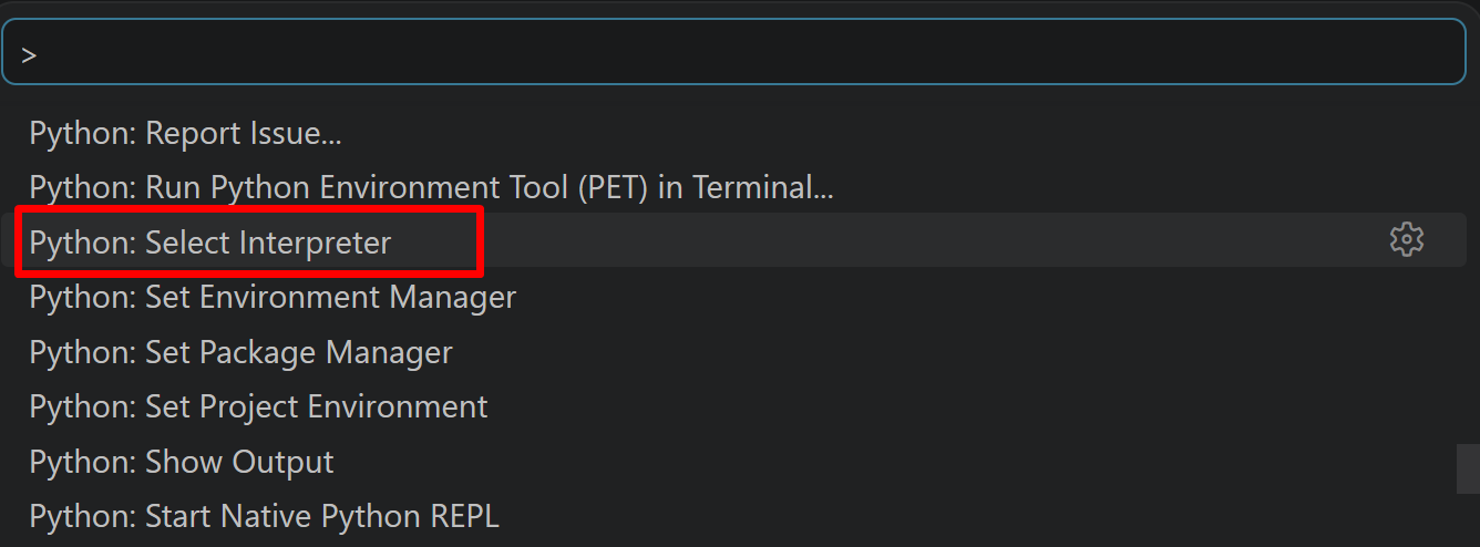
- 表示される一覧から,使用する Python(例:
C:\Program Files\Python312\python.exe)を選択する.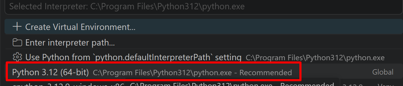
- パッケージのインポート,TensorFlow のバージョン確認など
from __future__ import absolute_import, division, print_function, unicode_literals
import tensorflow as tf
from tensorflow.keras import layers
from tensorflow.keras import backend as K
K.clear_session()
import numpy as np
import tensorflow_datasets as tfds
from tensorflow.keras.preprocessing import image

%matplotlib inline
import matplotlib.pyplot as plt
import warnings
warnings.filterwarnings('ignore')   # Suppress Matplotlib warnings

# TensorFlow のバージョン
print(tf.__version__)

# GPU を利用しているか
gpus = tf.config.list_physical_devices(device_type = 'GPU')
if len(gpus)>0:
    print(f">> GPU detected. {gpus[0].name}")
    tf.config.experimental.set_memory_growth(gpus[0], True)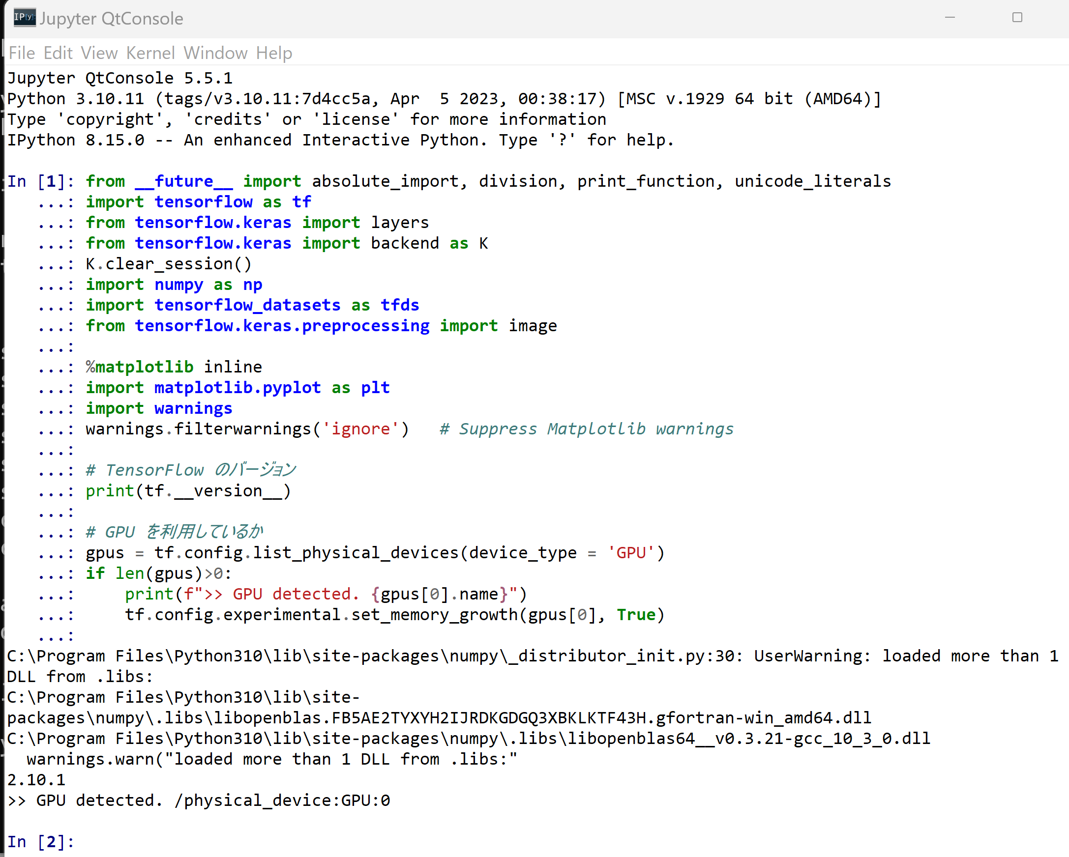
- CIFAR-10 データセットのロード
- x_train: サイズ 32 ×32 の 60000枚の濃淡画像
- y_train: 50000枚の濃淡画像それぞれの,種類番号(0 から 9 のどれか)
- x_test: サイズ 32 ×32 の 10000枚の濃淡画像
- y_test: 10000枚の濃淡画像それぞれの,種類番号(0 から 9 のどれか)
tensorflow_datasets の loadで, 「batch_size = -1」を指定して,一括読み込みを行っている.cifar10, cifar10_metadata = tfds.load('cifar10', with_info = True, shuffle_files=True, as_supervised=True, batch_size = -1) x_train, y_train, x_test, y_test = cifar10['train'][0], cifar10['train'][1], cifar10['test'][0], cifar10['test'][1] print(cifar10_metadata)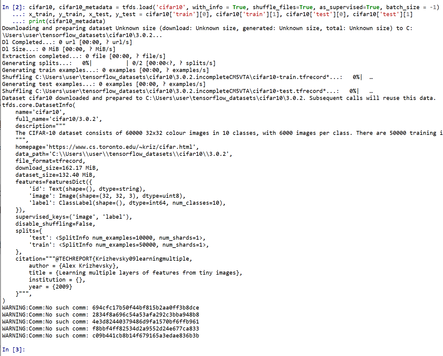
CIFAR-10 データセットの確認
- 型と形と最大値と最小値の確認
print(type(x_train), x_train.shape, np.max(x_train), np.min(x_train))
print(type(x_test), x_test.shape, np.max(x_test), np.min(x_test))
print(type(y_train), y_train.shape, np.max(y_train), np.min(y_train))
print(type(y_test), y_test.shape, np.max(y_test), np.min(y_test))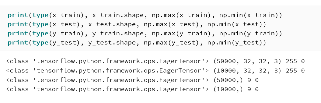
- データセットの中の画像を表示
MatplotLib を用いて,0 番目の画像を表示する
NUM = 0
plt.figure()
plt.imshow(x_train[NUM])
plt.colorbar()
plt.gca().grid(False)
plt.show()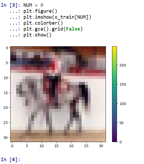
- データセットの情報を表示
print(cifar10_metadata)
print(cifar10_metadata.features["label"].num_classes)
print(cifar10_metadata.features["label"].names)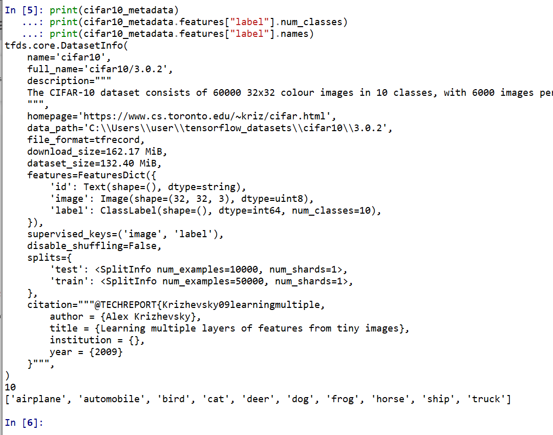
データの準備
- x_train, x_test, y_train, y_test の numpy ndarray への変換と,値の範囲の調整(値の範囲が 0 〜 255 であるのを,0 〜 1 に調整)
x_train = x_train.numpy().astype("float32") / 255.0
x_test = x_test.numpy().astype("float32") / 255.0
y_train = y_train.numpy()
y_test = y_test.numpy()
print(type(x_train), x_train.shape, np.max(x_train), np.min(x_train))
print(type(x_test), x_test.shape, np.max(x_test), np.min(x_test))
print(type(y_train), y_train.shape, np.max(y_train), np.min(y_train))
print(type(y_test), y_test.shape, np.max(y_test), np.min(y_test))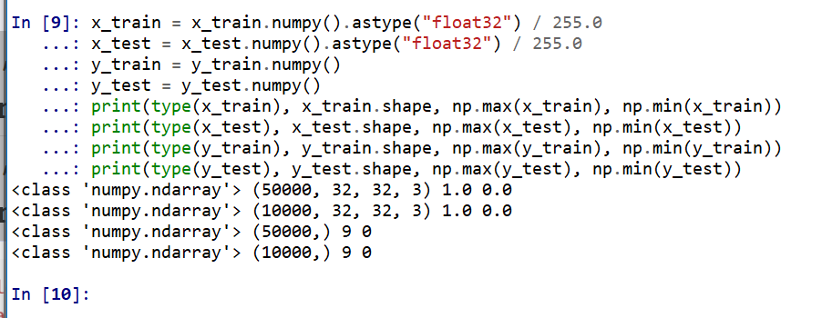
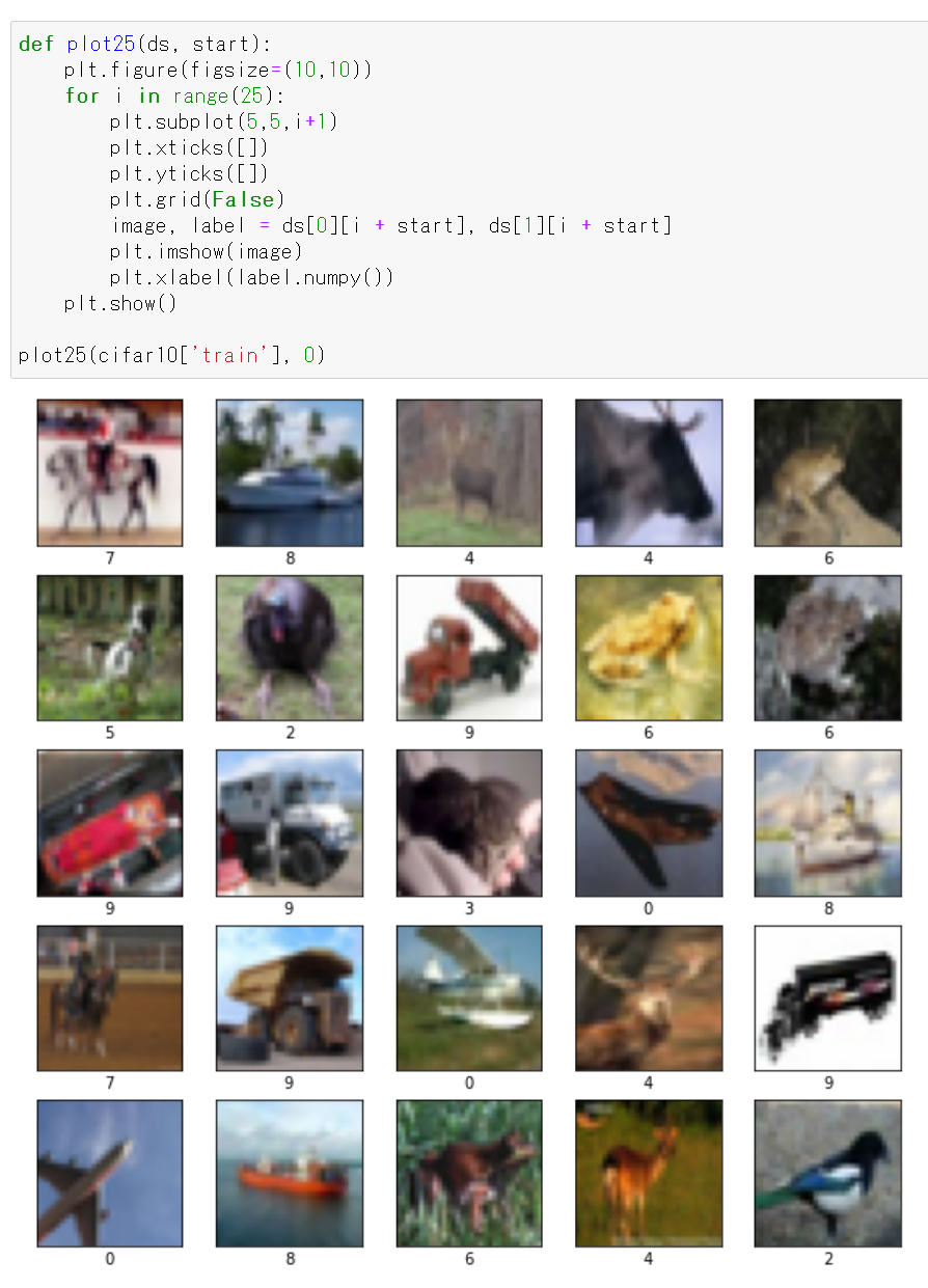
- データの確認表示
MatplotLib を用いて,複数の画像を並べて表示する.
plt.style.use('default')
plt.figure(figsize=(10,10))
for i in range(25):
  plt.subplot(5,5,i+1)
  plt.xticks([])
  plt.yticks([])
  plt.grid(False)
  plt.imshow(x_train[i], cmap=plt.cm.binary)
  plt.xlabel(y_train[i])

plt.show()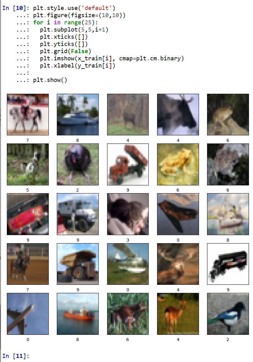
5. MobileNetV2 の作成,CIFAR-10 による学習,画像分類の実行
- ニューラルネットワークの作成
Keras の MobileNet を使う. 「weights=None」を指定することにより,最初,重みはランダムに設定する.
NUM_CLASSES = 10
input_shape = (32, 32, 3)
m1 = tf.keras.applications.mobilenet.MobileNet(input_shape=input_shape, weights=None, classes=NUM_CLASSES)
m1.summary()
m1.compile(
    optimizer=tf.keras.optimizers.Adam(learning_rate=0.001),
    loss='sparse_categorical_crossentropy',
    metrics=['sparse_categorical_crossentropy', 'accuracy'])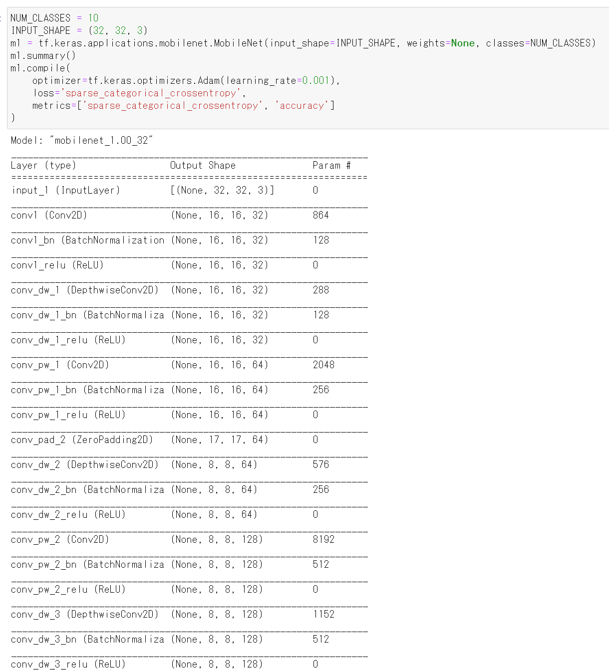
- モデルのビジュアライズ
Keras のモデルのビジュアライズについては: https://keras.io/ja/visualization/
ここでの表示で,エラーメッセージが出る場合でも,モデル自体は問題なくできていると考えられる.続行する.
from tensorflow.keras.utils import plot_model
import pydot
plot_model(m1)
- ニューラルネットワークの学習を行う
ニューラルネットワークの学習は fit メソッドにより行う. 教師データを使用する. 教師データを投入する.
epochs = 20
history = m1.fit(x_train, y_train,
                    epochs=epochs,
                    validation_data=(x_test, y_test),
                    verbose=1)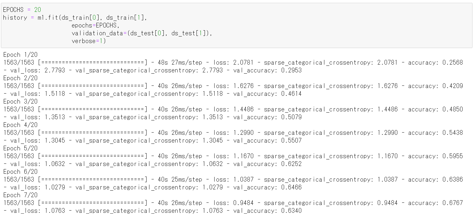
- CNN による画像分類
分類してみる.
print(m1.predict(x_test))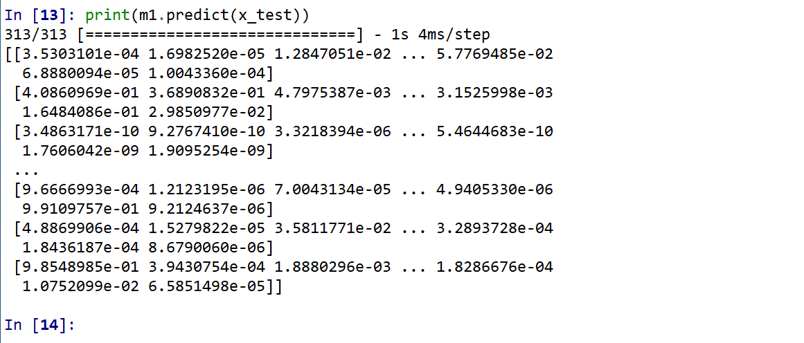
それぞれの数値の中で、一番大きいものはどれか?
m1.predict(x_test).argmax(axis=1)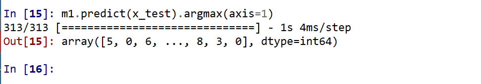
y_test 内にある正解のラベル(クラス名)を表示する(上の結果と比べるため)
print(y_test)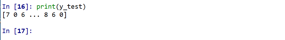
- 学習曲線の確認
過学習や学習不足について確認.
import pandas as pd
hist = pd.DataFrame(history.history)
hist['epoch'] = history.epoch
print(hist)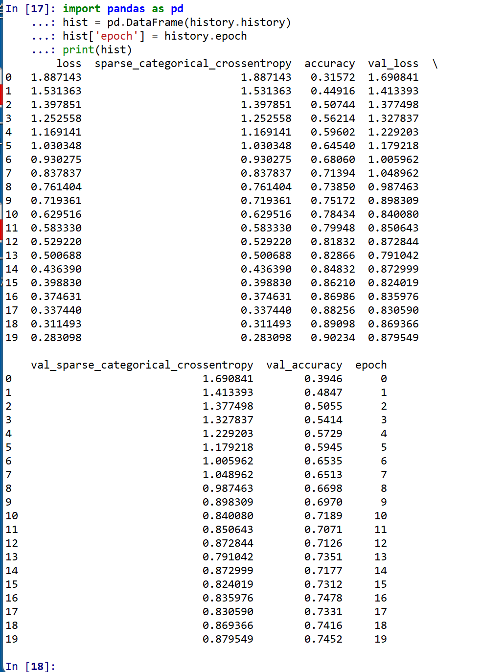
- 学習曲線のプロット
【関連する外部ページ】 訓練の履歴の可視化については,https://keras.io/ja/visualization/
- 学習時と検証時の,損失の違い
acc = history.history['accuracy']
val_acc = history.history['val_accuracy']
loss = history.history['loss']
val_loss = history.history['val_loss']

epochs = range(1, len(acc) + 1)

# "bo" は青いドット
plt.plot(epochs, loss, 'bo', label='Training loss')
# ”b" は青い実線
plt.plot(epochs, val_loss, 'b', label='Validation loss')
plt.title('Training and validation loss')
plt.xlabel('Epochs')
plt.ylabel('Loss')
plt.legend()

plt.show()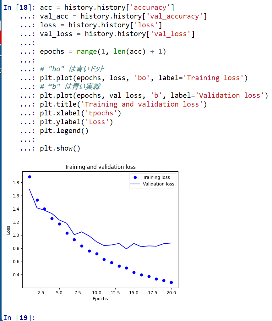
- 学習時と検証時の,精度の違い
acc = history.history['accuracy']
val_acc = history.history['val_accuracy']
loss = history.history['loss']
val_loss = history.history['val_loss']

plt.clf()   # 図のクリア
plt.plot(epochs, acc, 'bo', label='Training acc')
plt.plot(epochs, val_acc, 'b', label='Validation acc')
plt.title('Training and validation accuracy')
plt.xlabel('Epochs')
plt.ylabel('Accuracy')
plt.legend()

plt.show()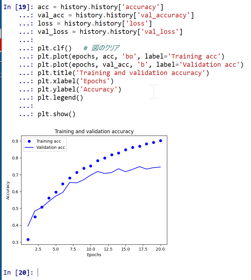
6. ResNet50 の作成,CIFAR-10 による学習,画像分類の実行
- ニューラルネットワークの作成
Keras の ResNet50 を使う. 「weights=None」を指定することにより,最初,重みはランダムに設定する.
NUM_CLASSES = 10
input_shape = (32, 32, 3)
m2 = tf.keras.applications.resnet50.ResNet50(input_shape=input_shape, weights=None, classes=NUM_CLASSES)
m2.summary()
m2.compile(
    optimizer=tf.keras.optimizers.Adam(learning_rate=0.001),
    loss='sparse_categorical_crossentropy',
    metrics=['sparse_categorical_crossentropy', 'accuracy'])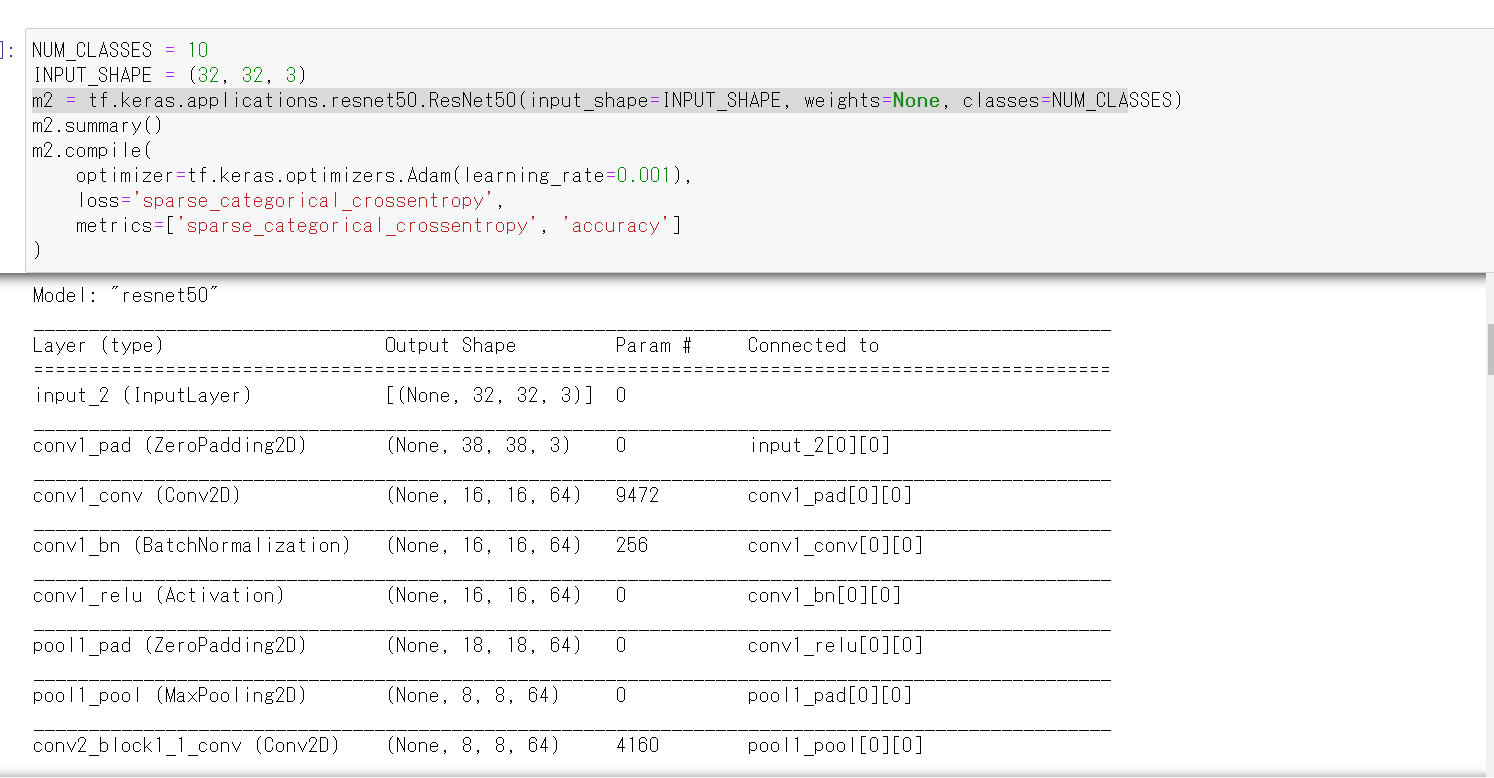
- モデルのビジュアライズ
Keras のモデルのビジュアライズについては: https://keras.io/ja/visualization/
ここでの表示で,エラーメッセージが出る場合でも,モデル自体は問題なくできていると考えられる.続行する.
from tensorflow.keras.utils import plot_model
import pydot
plot_model(m2)
- ニューラルネットワークの学習を行う
ニューラルネットワークの学習は fit メソッドにより行う. 教師データを使用する. 教師データを投入する.
epochs = 20
history = m2.fit(x_train, y_train,
                    epochs=epochs,
                    validation_data=(x_test, y_test),
                    verbose=1)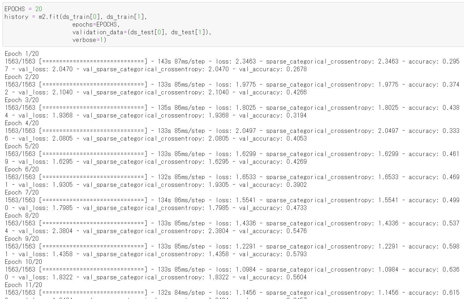
- CNN による画像分類
分類してみる.
print(m2.predict(x_test))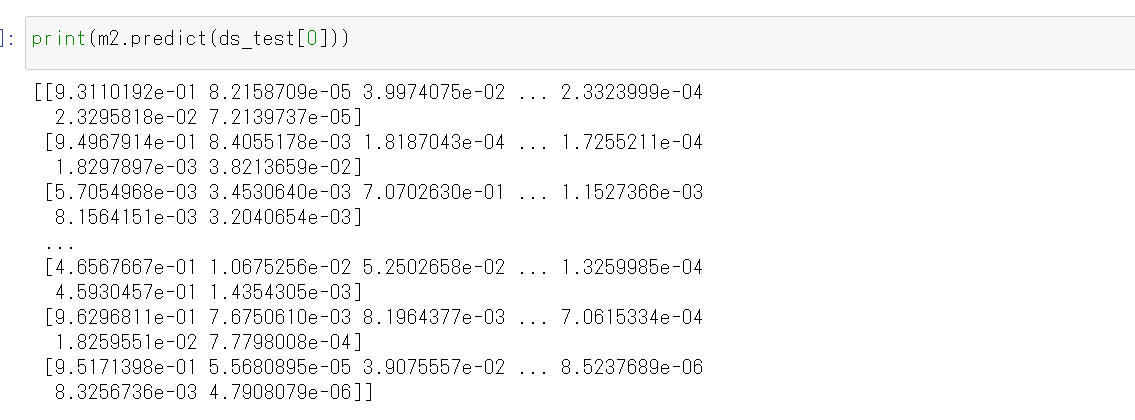
それぞれの数値の中で、一番大きいものはどれか?
m2.predict(x_test).argmax(axis=1)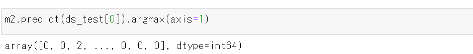
y_test 内にある正解のラベル(クラス名)を表示する(上の結果と比べるため)
print(y_test)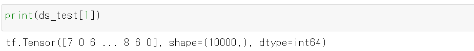
- 学習曲線の確認
過学習や学習不足について確認.
import pandas as pd
hist = pd.DataFrame(history.history)
hist['epoch'] = history.epoch
print(hist)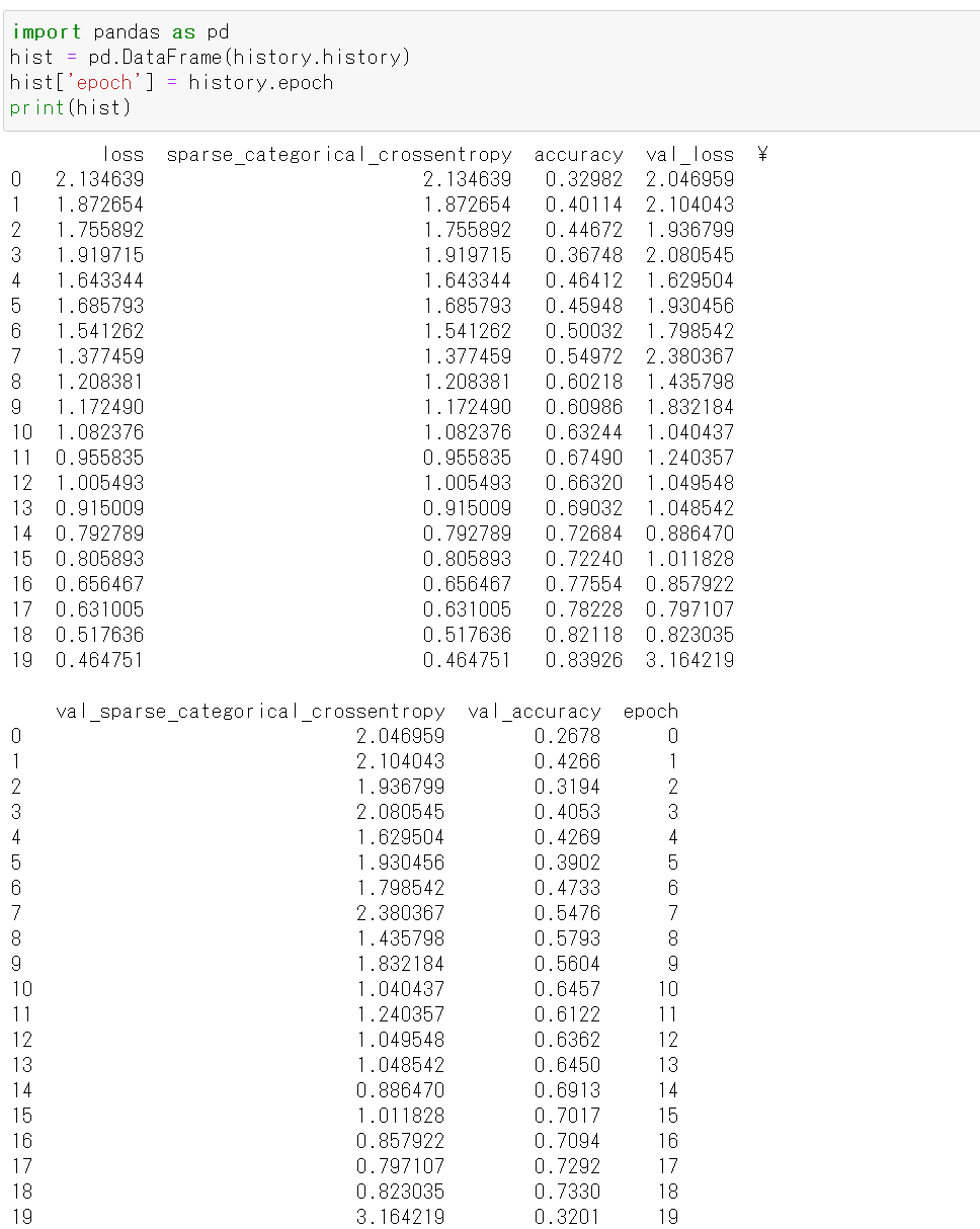
- 学習曲線のプロット
【関連する外部ページ】 訓練の履歴の可視化については,https://keras.io/ja/visualization/
- 学習時と検証時の,損失の違い
acc = history.history['accuracy']
val_acc = history.history['val_accuracy']
loss = history.history['loss']
val_loss = history.history['val_loss']

epochs = range(1, len(acc) + 1)

# "bo" は青いドット
plt.plot(epochs, loss, 'bo', label='Training loss')
# ”b" は青い実線
plt.plot(epochs, val_loss, 'b', label='Validation loss')
plt.title('Training and validation loss')
plt.xlabel('Epochs')
plt.ylabel('Loss')
plt.legend()

plt.show()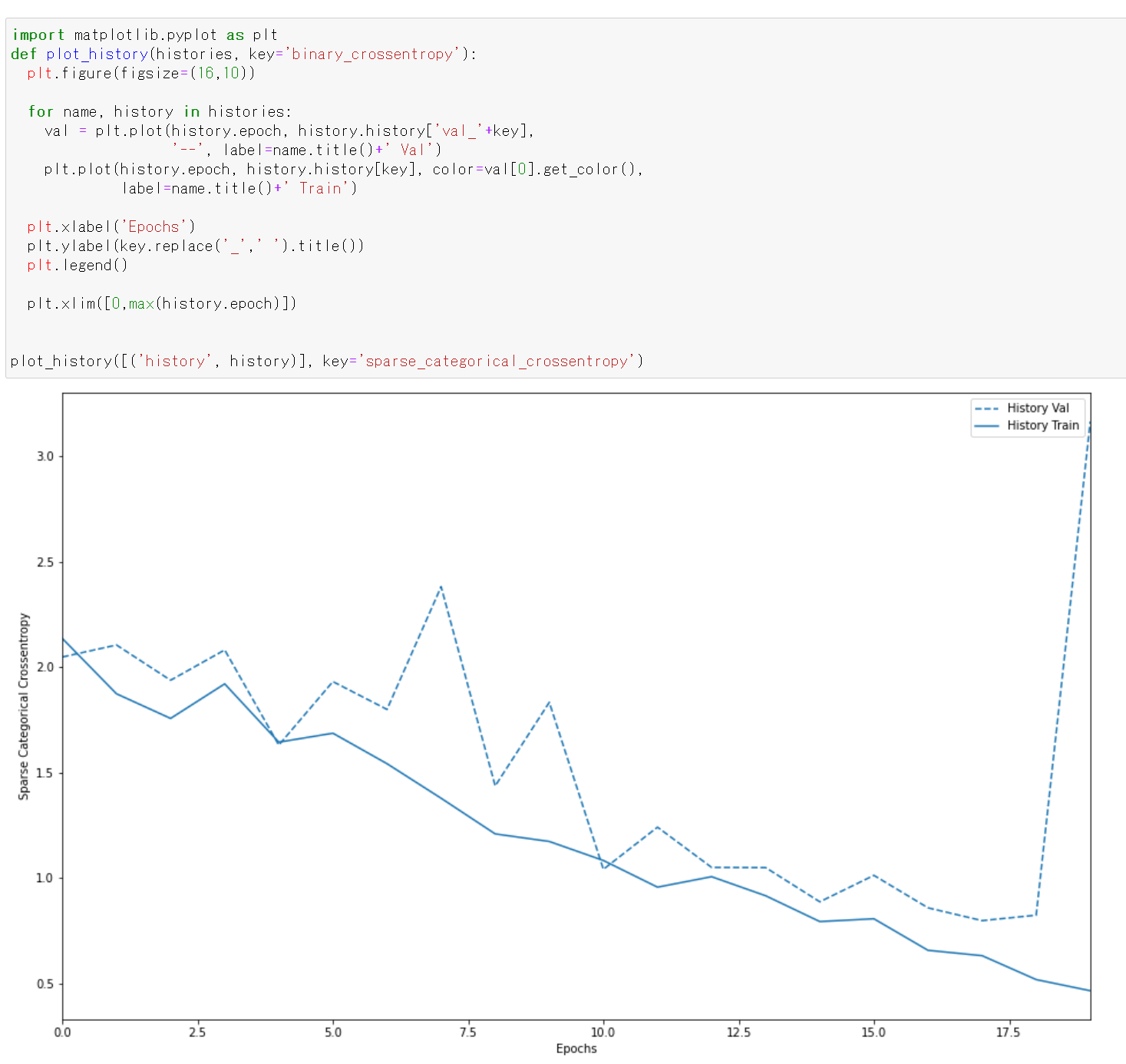
- 学習時と検証時の,精度の違い
acc = history.history['accuracy']
val_acc = history.history['val_accuracy']
loss = history.history['loss']
val_loss = history.history['val_loss']

plt.clf()   # 図のクリア
plt.plot(epochs, acc, 'bo', label='Training acc')
plt.plot(epochs, val_acc, 'b', label='Validation acc')
plt.title('Training and validation accuracy')
plt.xlabel('Epochs')
plt.ylabel('Accuracy')
plt.legend()

plt.show()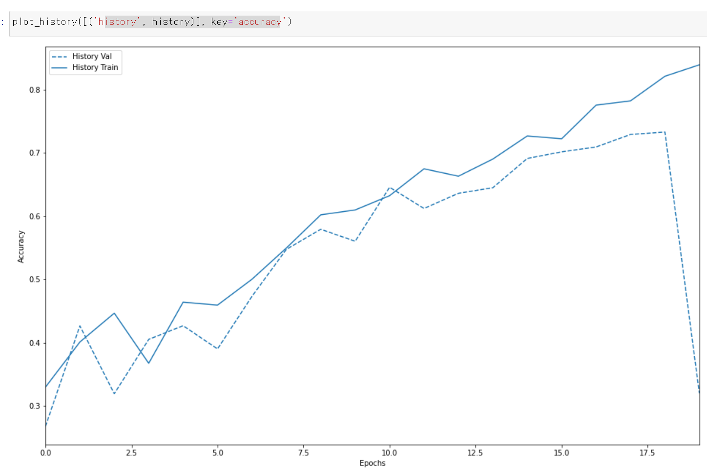
9. ニューラルネットワークの作成(DenseNet 121 を使用)
- ニューラルネットワークの作成と確認とコンパイル
Keras の DenseNet121 を使う. 「weights=None」を指定することにより,最初,重みはランダムに設定する.
NUM_CLASSES = 10
input_shape = (32, 32, 3)
m3 = tf.keras.applications.densenet.DenseNet121(input_shape=input_shape, weights=None, classes=NUM_CLASSES)
m3.summary()
m3.compile(
    optimizer=tf.keras.optimizers.Adam(learning_rate=0.001),
    loss='sparse_categorical_crossentropy',
    metrics=['sparse_categorical_crossentropy', 'accuracy'])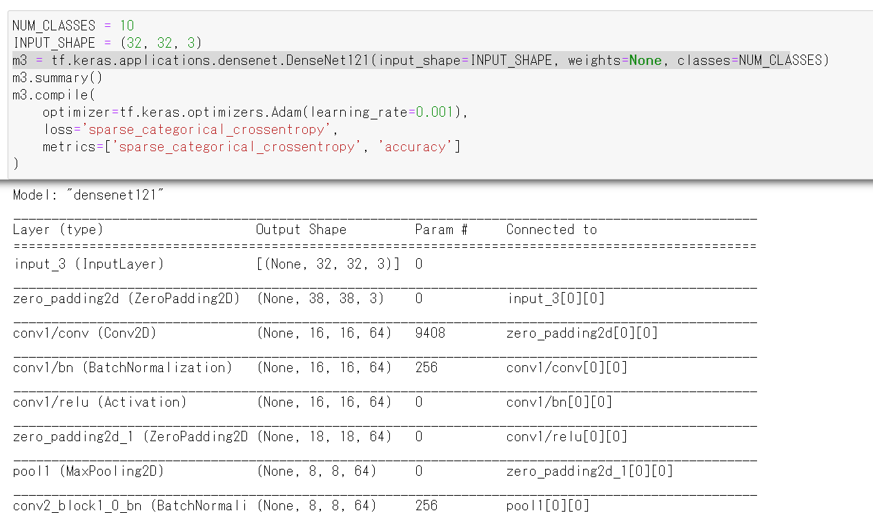
- モデルのビジュアライズ
Keras のモデルのビジュアライズについては: https://keras.io/ja/visualization/
ここでの表示で,エラーメッセージが出る場合でも,モデル自体は問題なくできていると考えられる.続行する.
from tensorflow.keras.utils import plot_model
import pydot
plot_model(m3)
10. ニューラルネットワークの学習(DenseNet 121 を使用)
- ニューラルネットワークの学習を行う
ニューラルネットワークの学習は fit メソッドにより行う. 教師データを使用する. 教師データを投入する.
epochs = 20
history = m3.fit(x_train, y_train,
                    epochs=epochs,
                    validation_data=(x_test, y_test),
                    verbose=1)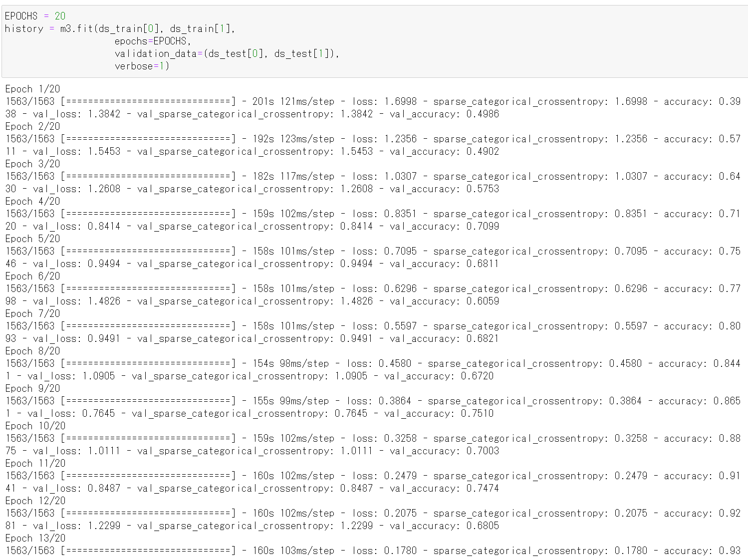
- CNN による画像分類
分類してみる.
print(m3.predict(x_test))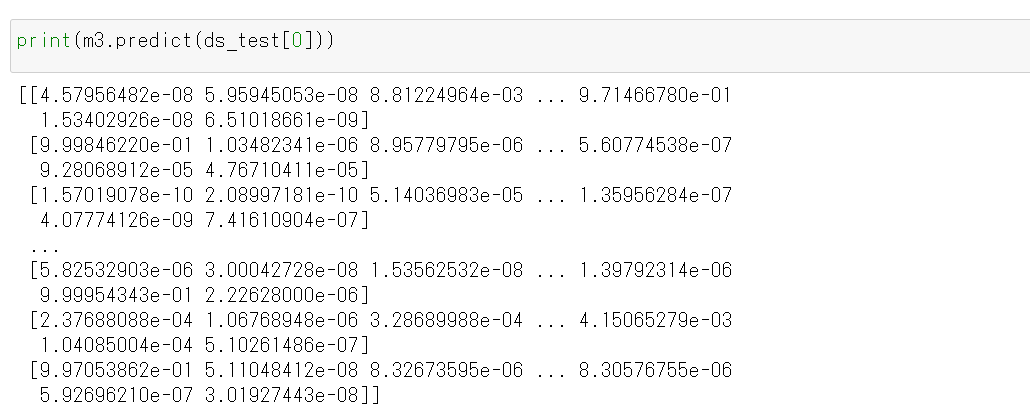
それぞれの数値の中で、一番大きいものはどれか?
m3.predict(x_test).argmax(axis=1)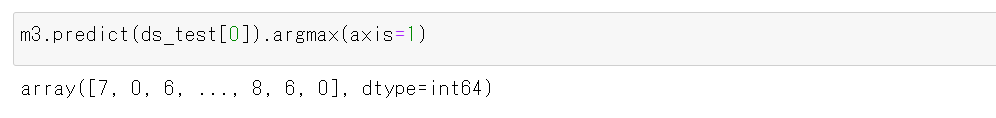
y_test 内にある正解のラベル(クラス名)を表示する(上の結果と比べるため)
print(y_test)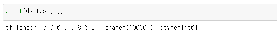
- 学習曲線の確認
過学習や学習不足について確認.
import pandas as pd
hist = pd.DataFrame(history.history)
hist['epoch'] = history.epoch
print(hist)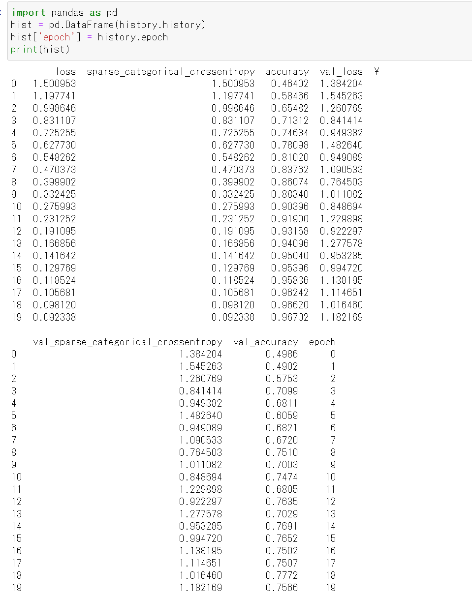
- 学習曲線のプロット
過学習や学習不足について確認.
https://www.tensorflow.org/tutorials/keras/overfit_and_underfit?hl=ja で公開されているプログラムを使用
%matplotlib inline
import matplotlib.pyplot as plt
import warnings
warnings.filterwarnings('ignore')   # Suppress Matplotlib warnings
def plot_history(histories, key='binary_crossentropy'):
  plt.figure(figsize=(16,10))

  for name, history in histories:
    val = plt.plot(history.epoch, history.history['val_'+key],
                   '--', label=name.title()+' Val')
    plt.plot(history.epoch, history.history[key], color=val[0].get_color(),
             label=name.title()+' Train')

  plt.xlabel('Epochs')
  plt.ylabel(key.replace('_',' ').title())
  plt.legend()

  plt.xlim([0,max(history.epoch)])


plot_history([('history', history)], key='sparse_categorical_crossentropy')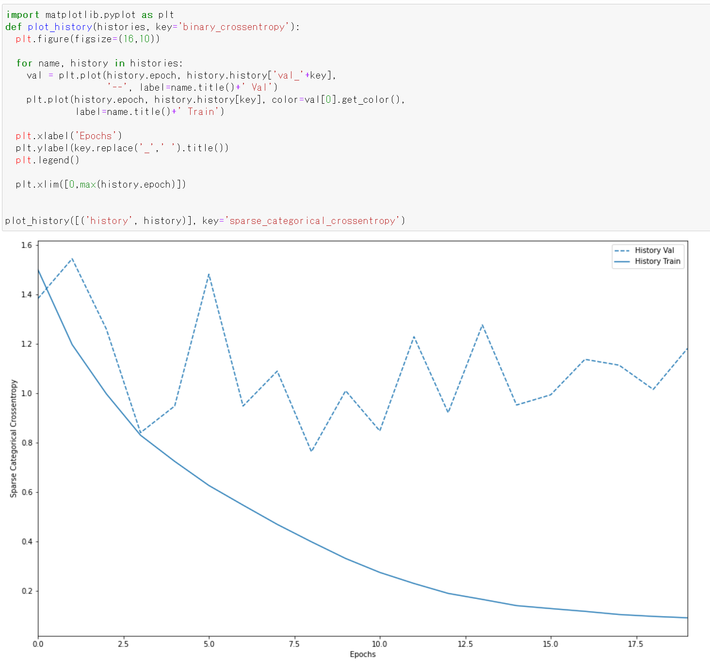
plot_history([('history', history)], key='accuracy')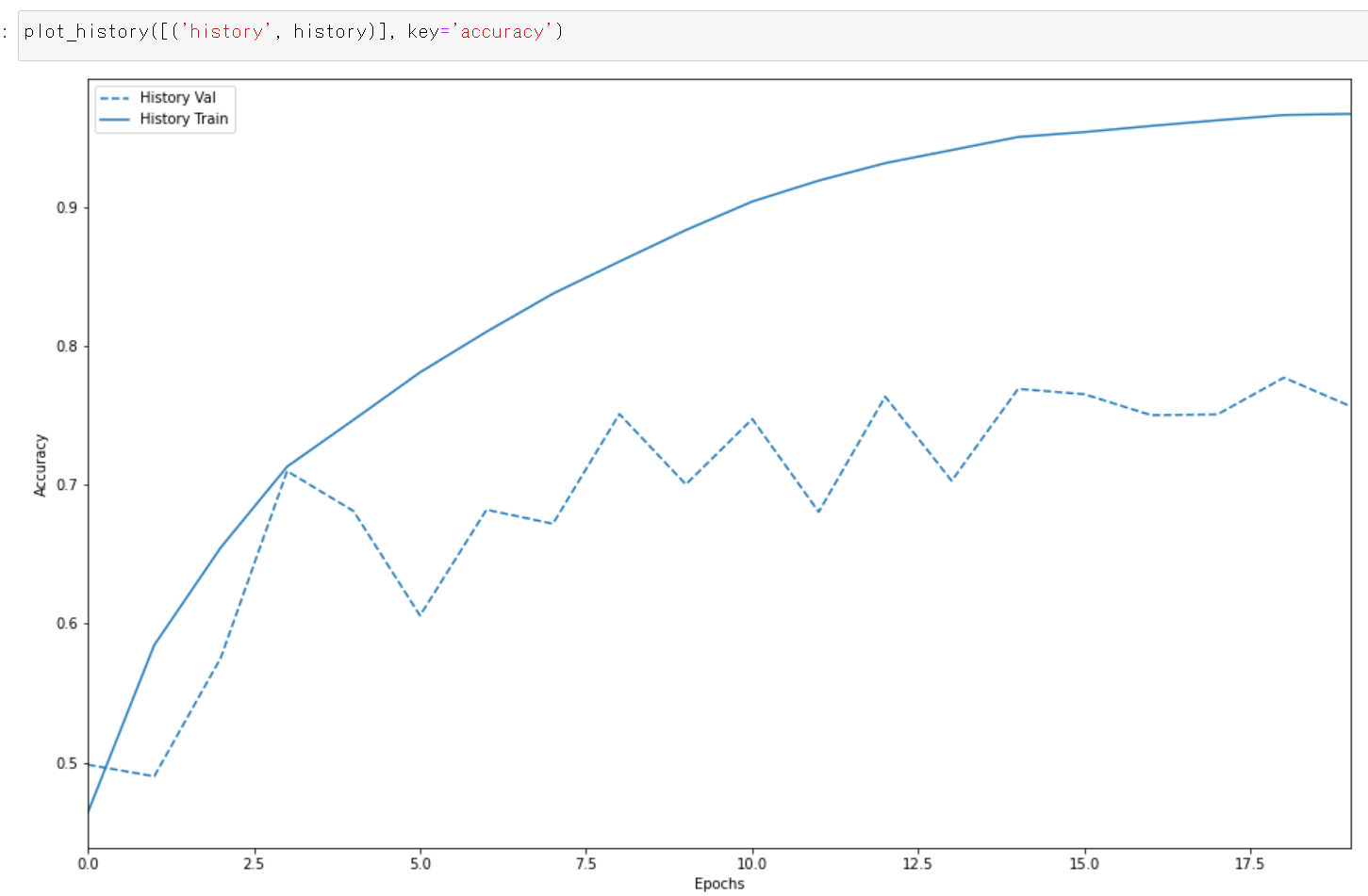
11. ニューラルネットワークの作成(DenseNet 169 を使用)
- ニューラルネットワークの作成と確認とコンパイル
Keras の DenseNet169 を使う. 「weights=None」を指定することにより,最初,重みはランダムに設定する.
NUM_CLASSES = 10
input_shape = (32, 32, 3)
m4 = tf.keras.applications.densenet.DenseNet169(input_shape=input_shape, weights=None, classes=NUM_CLASSES)
m4.summary()
m4.compile(
    optimizer=tf.keras.optimizers.Adam(learning_rate=0.001),
    loss='sparse_categorical_crossentropy',
    metrics=['sparse_categorical_crossentropy', 'accuracy'])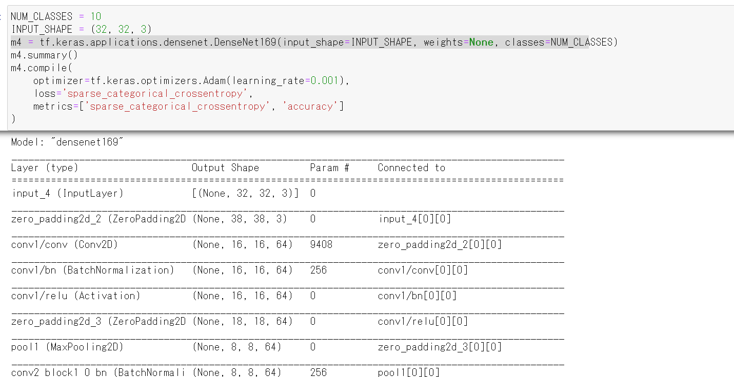
- モデルのビジュアライズ
Keras のモデルのビジュアライズについては: https://keras.io/ja/visualization/
ここでの表示で,エラーメッセージが出る場合でも,モデル自体は問題なくできていると考えられる.続行する.
from tensorflow.keras.utils import plot_model
import pydot
plot_model(m4)
12. ニューラルネットワークの学習(DenseNet 169 を使用)
- ニューラルネットワークの学習を行う
ニューラルネットワークの学習は fit メソッドにより行う. 教師データを使用する. 教師データを投入する.
epochs = 20
history = m4.fit(x_train, y_train,
                    epochs=epochs,
                    validation_data=(x_test, y_test),
                    verbose=1)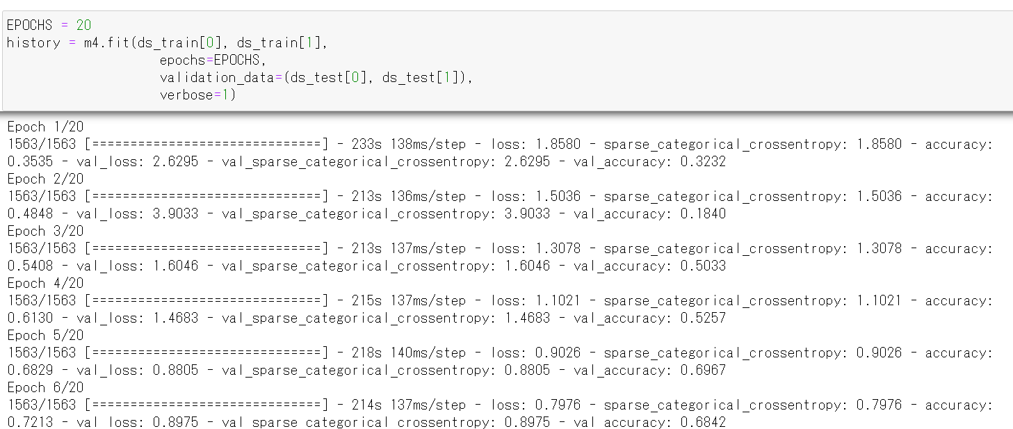
- CNN による画像分類
分類してみる.
print(m4.predict(x_test))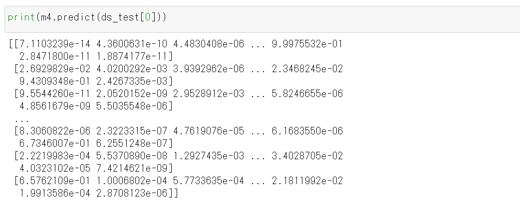
それぞれの数値の中で、一番大きいものはどれか?
m4.predict(x_test).argmax(axis=1)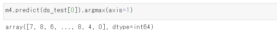
y_test 内にある正解のラベル(クラス名)を表示する(上の結果と比べるため)
print(y_test)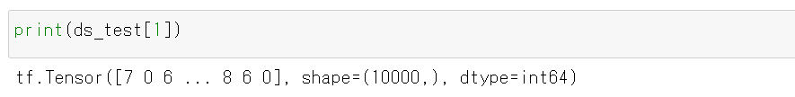
- 学習曲線の確認
過学習や学習不足について確認.
import pandas as pd
hist = pd.DataFrame(history.history)
hist['epoch'] = history.epoch
print(hist)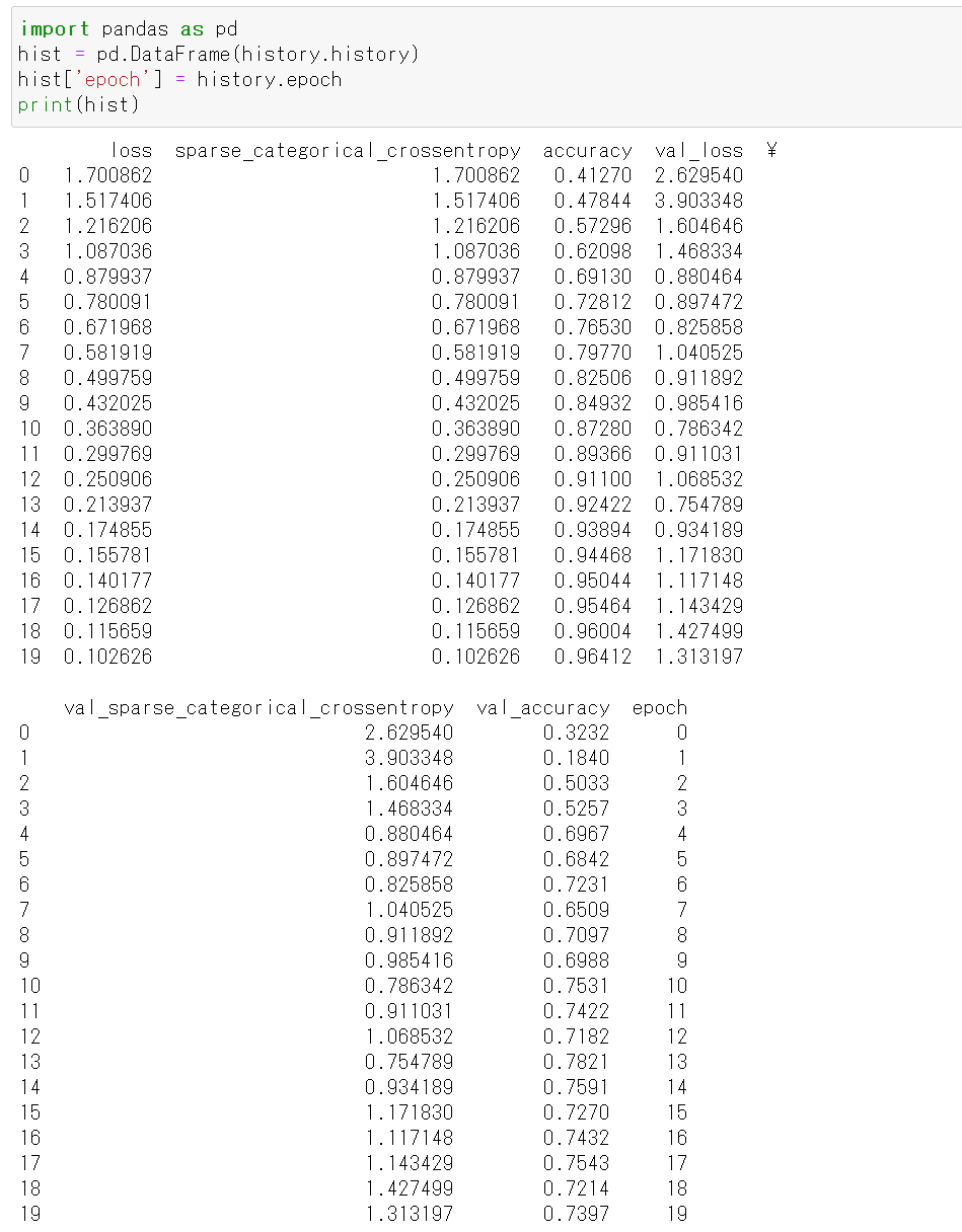
- 学習曲線のプロット
過学習や学習不足について確認.
https://www.tensorflow.org/tutorials/keras/overfit_and_underfit?hl=ja で公開されているプログラムを使用
%matplotlib inline
import matplotlib.pyplot as plt
import warnings
warnings.filterwarnings('ignore')   # Suppress Matplotlib warnings
def plot_history(histories, key='binary_crossentropy'):
  plt.figure(figsize=(16,10))

  for name, history in histories:
    val = plt.plot(history.epoch, history.history['val_'+key],
                   '--', label=name.title()+' Val')
    plt.plot(history.epoch, history.history[key], color=val[0].get_color(),
             label=name.title()+' Train')

  plt.xlabel('Epochs')
  plt.ylabel(key.replace('_',' ').title())
  plt.legend()

  plt.xlim([0,max(history.epoch)])


plot_history([('history', history)], key='sparse_categorical_crossentropy')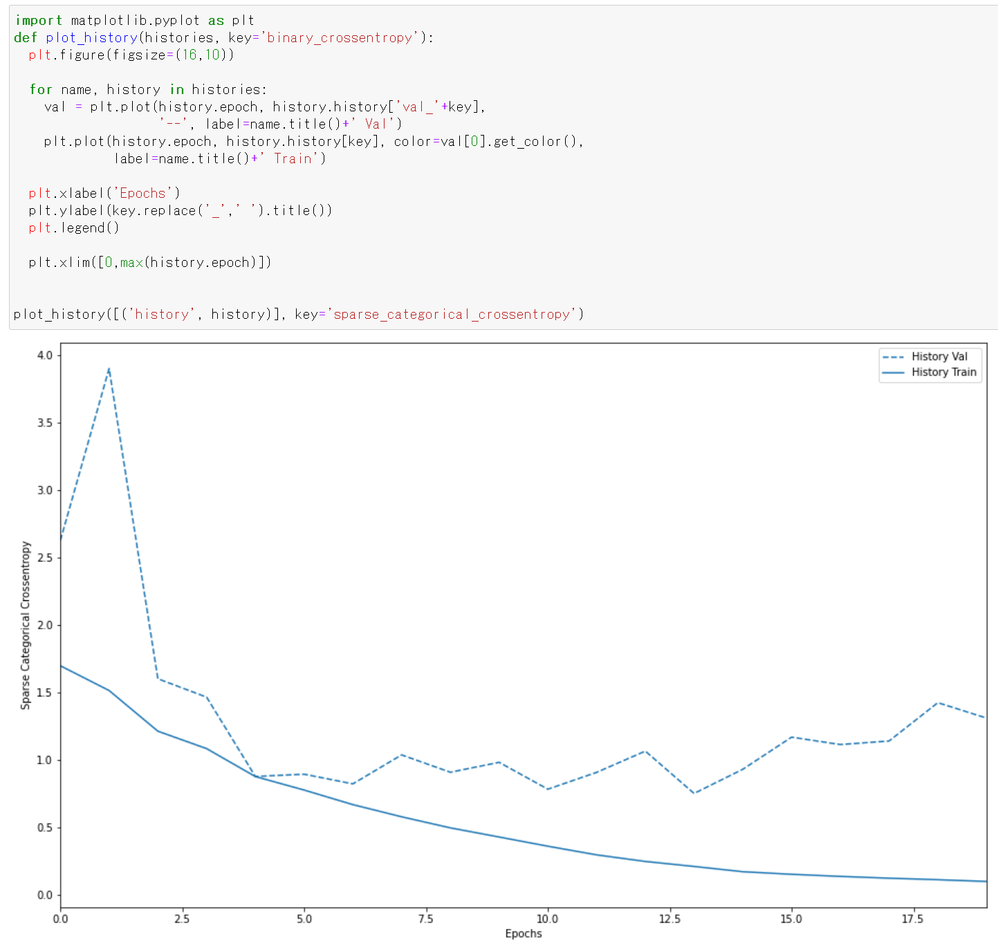
plot_history([('history', history)], key='accuracy')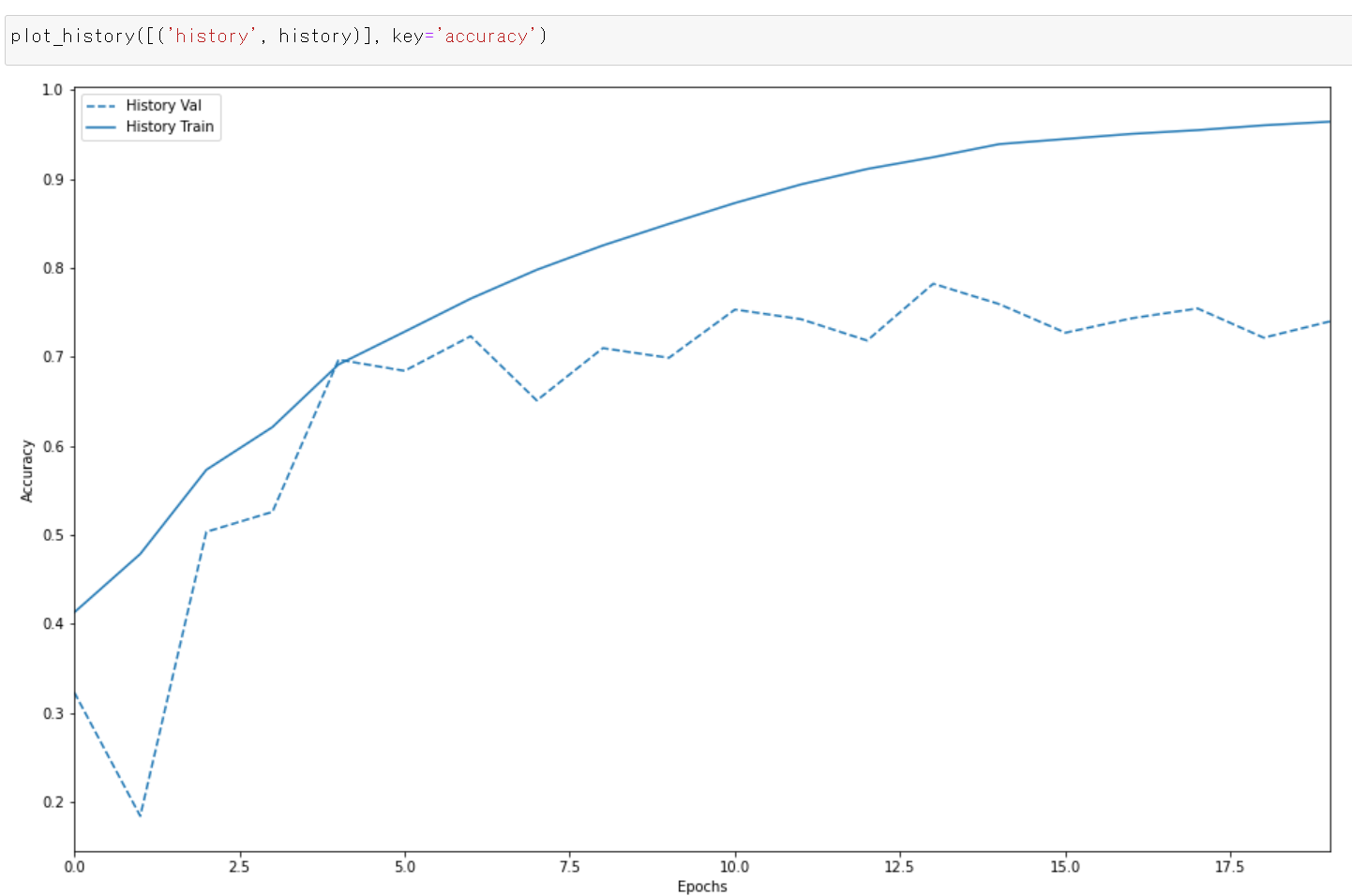
13. ニューラルネットワークの作成(NASNet を使用)
- ニューラルネットワークの作成と確認とコンパイル
NUM_CLASSES = 10
input_shape = (32, 32, 3)
m5 = tf.keras.applications.nasnet.NASNetMobile(input_shape=input_shape, weights=None, classes=NUM_CLASSES)
m5.summary()
m5.compile(
    optimizer=tf.keras.optimizers.Adam(learning_rate=0.001),
    loss='sparse_categorical_crossentropy',
    metrics=['sparse_categorical_crossentropy', 'accuracy'])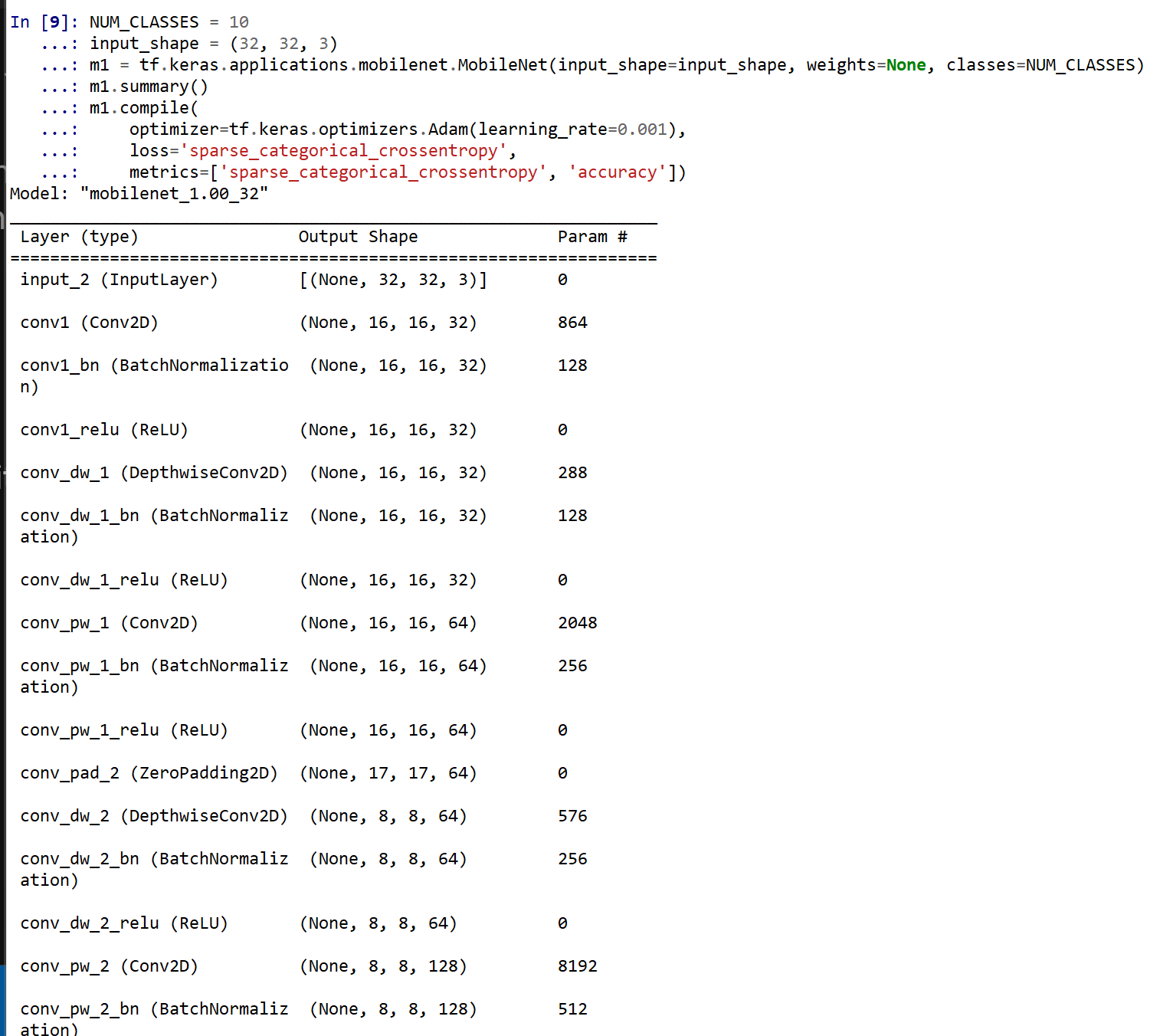
- モデルのビジュアライズ
Keras のモデルのビジュアライズについては: https://keras.io/ja/visualization/
ここでの表示で,エラーメッセージが出る場合でも,モデル自体は問題なくできていると考えられる.続行する.
from tensorflow.keras.utils import plot_model
import pydot
plot_model(m5)
14. ニューラルネットワークの学習(NASNet を使用)
- ニューラルネットワークの学習を行う
ニューラルネットワークの学習は fit メソッドにより行う. 教師データを使用する. 教師データを投入する.
epochs = 20
history = m5.fit(x_train, y_train,
                    epochs=epochs,
                    validation_data=(x_test, y_test),
                    verbose=1)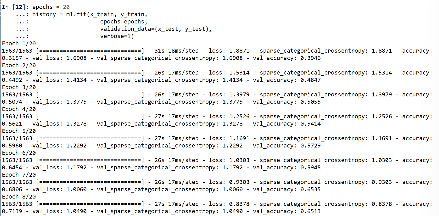
- CNN による画像分類
分類してみる.
print(m5.predict(x_test))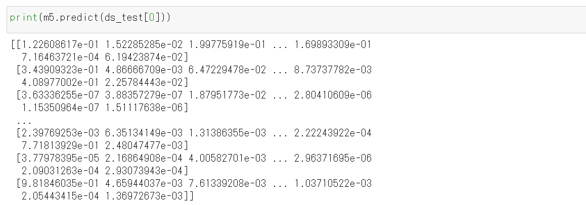
それぞれの数値の中で、一番大きいものはどれか?
cvm5.predict(x_test).argmax(axis=1)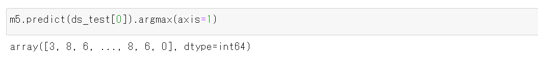
y_test 内にある正解のラベル(クラス名)を表示する(上の結果と比べるため)
print(y_test)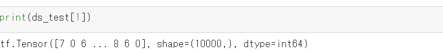
- 学習曲線の確認
過学習や学習不足について確認.
import pandas as pd
hist = pd.DataFrame(history.history)
hist['epoch'] = history.epoch
print(hist)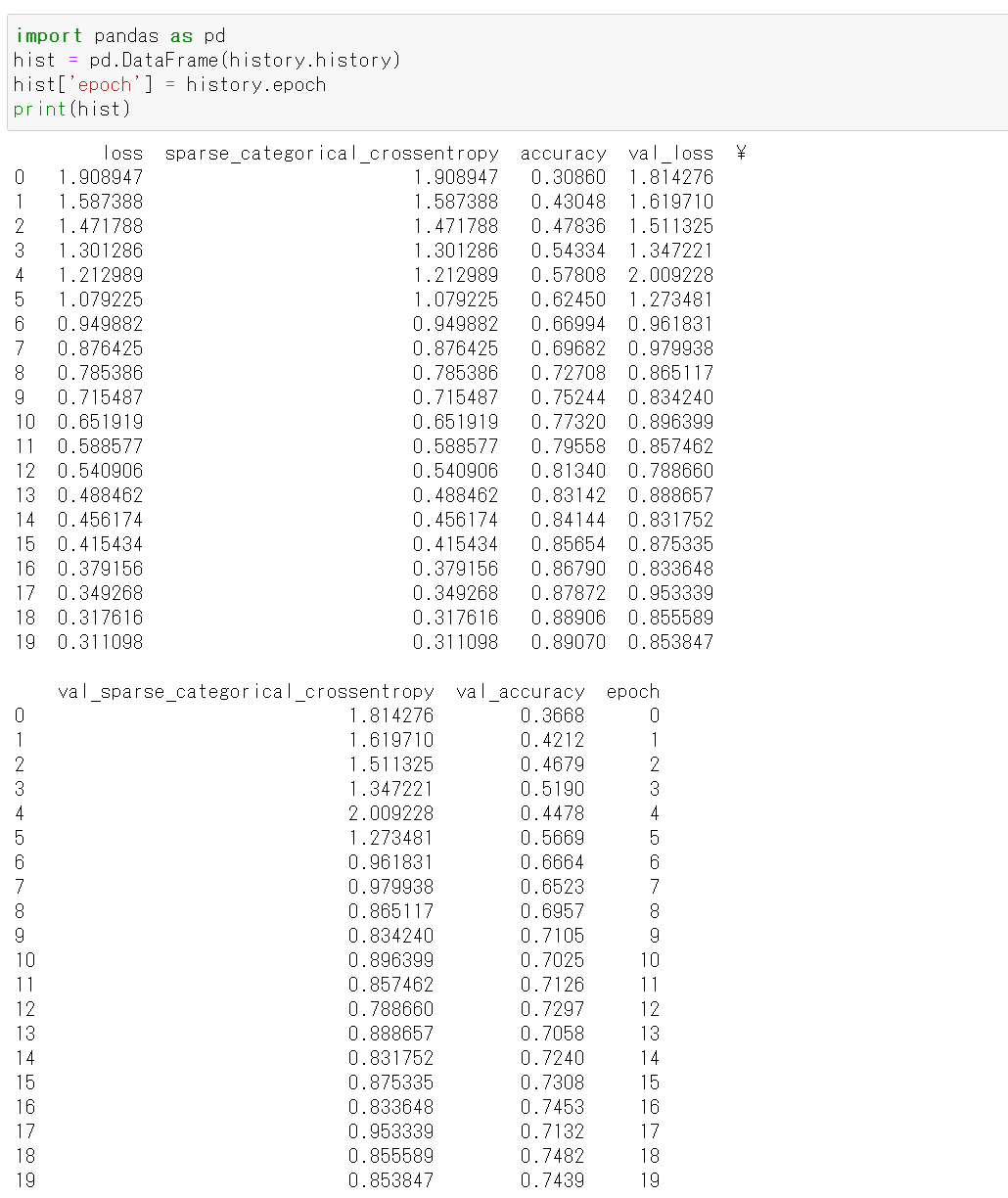
- 学習曲線のプロット
過学習や学習不足について確認.
https://www.tensorflow.org/tutorials/keras/overfit_and_underfit?hl=ja で公開されているプログラムを使用
%matplotlib inline
import matplotlib.pyplot as plt
import warnings
warnings.filterwarnings('ignore')   # Suppress Matplotlib warnings
def plot_history(histories, key='binary_crossentropy'):
  plt.figure(figsize=(16,10))

  for name, history in histories:
    val = plt.plot(history.epoch, history.history['val_'+key],
                   '--', label=name.title()+' Val')
    plt.plot(history.epoch, history.history[key], color=val[0].get_color(),
             label=name.title()+' Train')

  plt.xlabel('Epochs')
  plt.ylabel(key.replace('_',' ').title())
  plt.legend()

  plt.xlim([0,max(history.epoch)])


plot_history([('history', history)], key='sparse_categorical_crossentropy')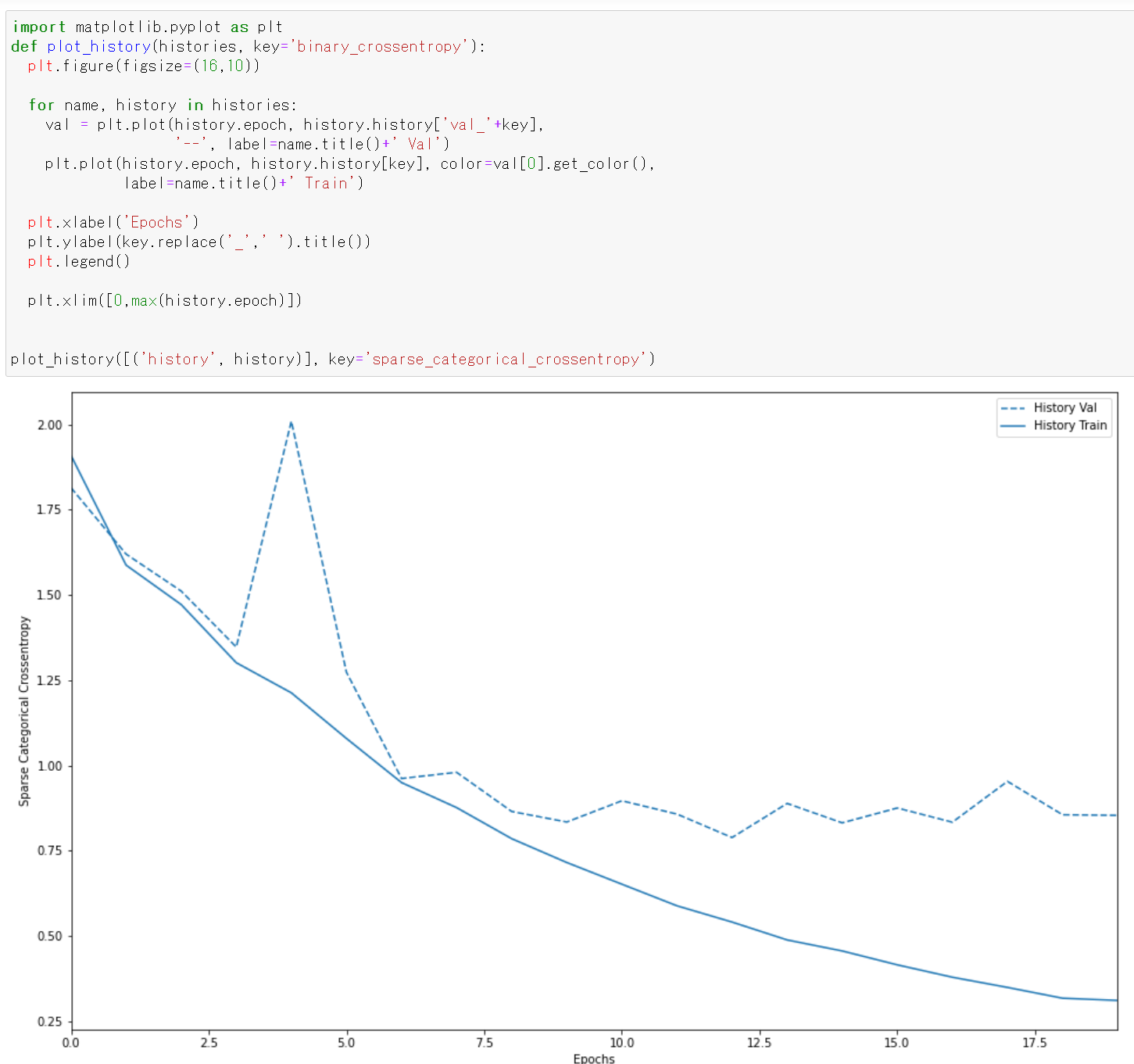
plot_history([('history', history)], key='accuracy')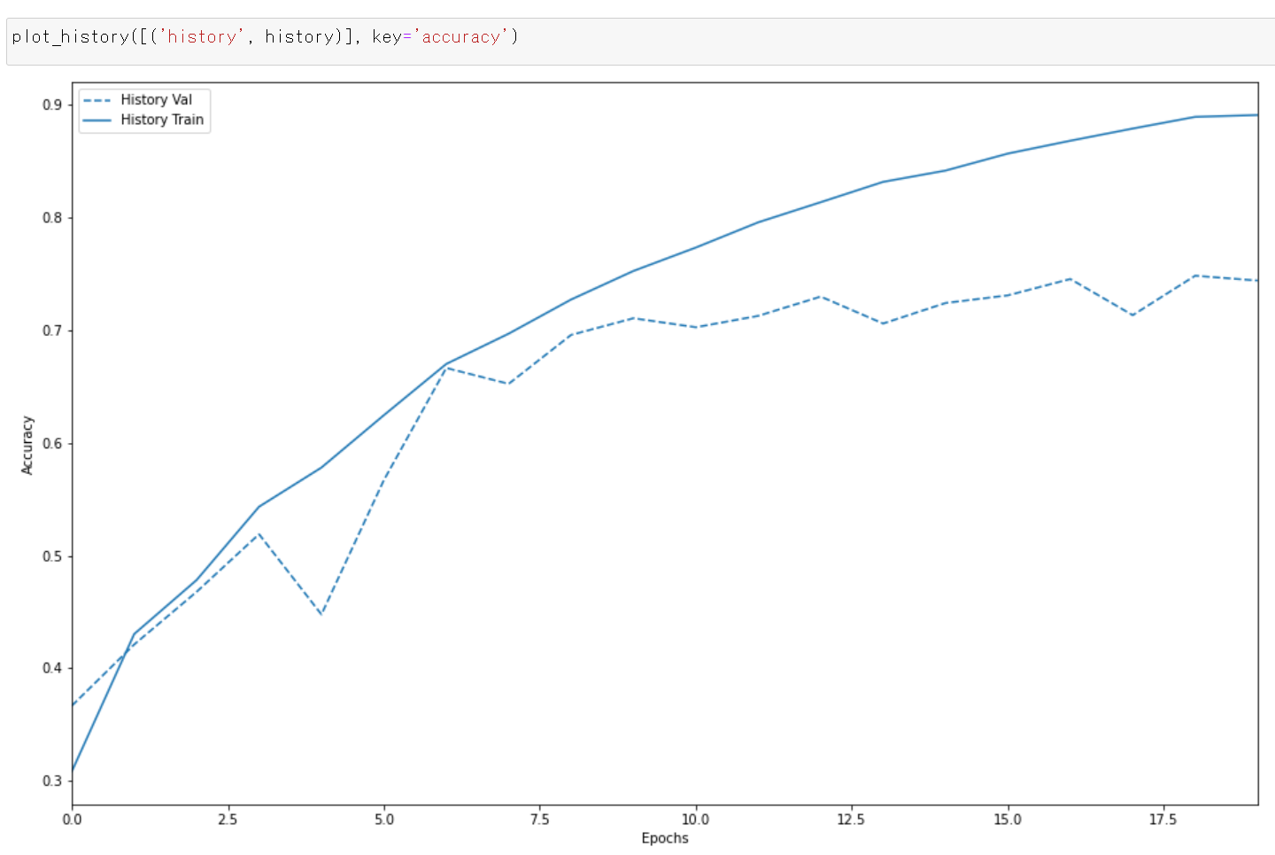
- ニューラルネットワークの学習を行う
- ニューラルネットワークの学習を行う
- ニューラルネットワークの学習を行う
- ニューラルネットワークの学習を行う
- ニューラルネットワークの学習を行う