階層クラスタリング（数値ベクトルの集合）(a set of numeric vectors)

サンプルデータ

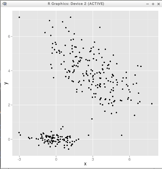
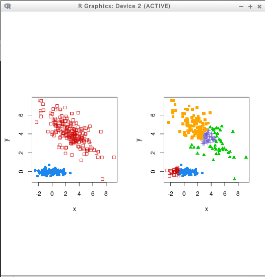
* サンプルデータ２次元

• cluster #1: center(0,0), N=100, vec=(1,0)
• cluster #2: center(3,4), N=200, vec=(2,-1)

require(data.table)
require(ggplot2)

x1 <- rnorm(100)
y1 <- rnorm(100) * 0.2

a2 <- rnorm(200)
b2 <- rnorm(200) * 0.4
x2 <- a2 * 2 + b2 + 3
y2 <- - a2 + 2 * b2 + 4

D <- data.table( x=c(x1,x2), y=c(y1,y2) )
p <- ggplot(D, aes(x = x, y = y))
p + geom_point(size = 2)

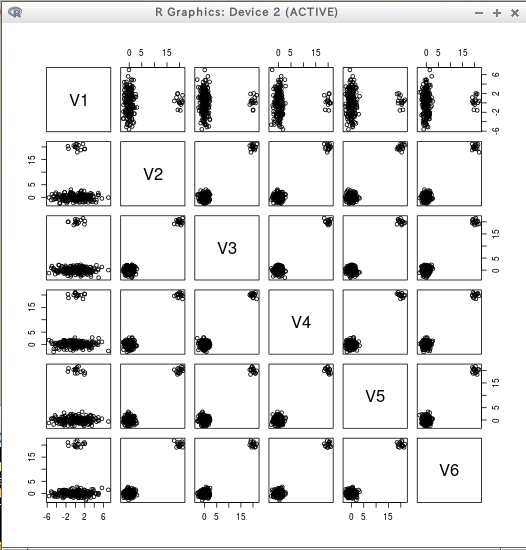
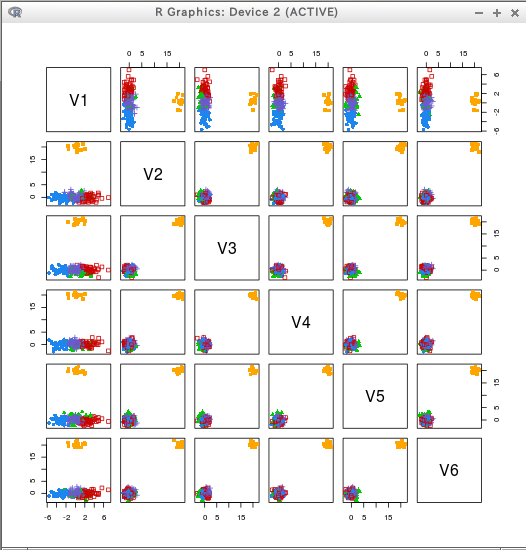
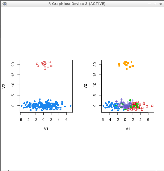
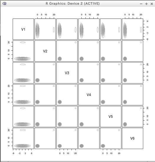
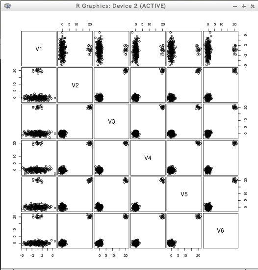
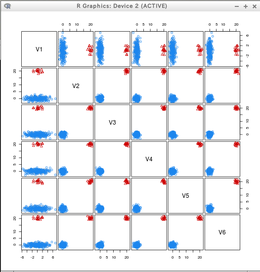
* サンプルデータ６次元

require(data.table)
require(ggplot2)
require(mvtnorm)

T <- data.table( rbind(rmvnorm(200, rep(0, 6), diag(c(5, rep(1,5)))),
     rmvnorm( 15, c(0, rep(20, 5)), diag(rep(1, 6)))) )
plot(T)

階層クラスタリング　(hierarchical clustering)

mclust パッケージの Mclust() 関数を用いたクラスタリング (clusering using Mclust() in the mclust package)

1. 準備

   install.packages("mclust")
   

2. クラスタリング結果のプロット (plot clustering result)

   * テストデータ

   require(mclust)
   C = Mclust(D)
   summary(C)
   plot(C)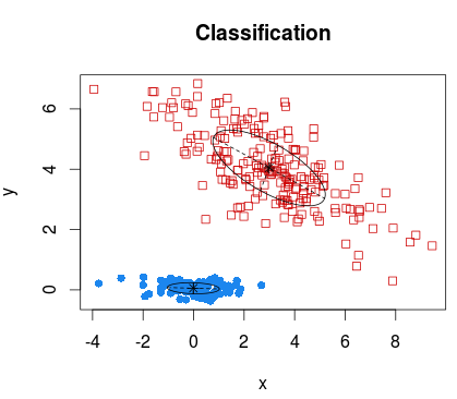
   

   

   require(mclust)
   C2 = Mclust(T)
   summary(C2)
   plot(C2)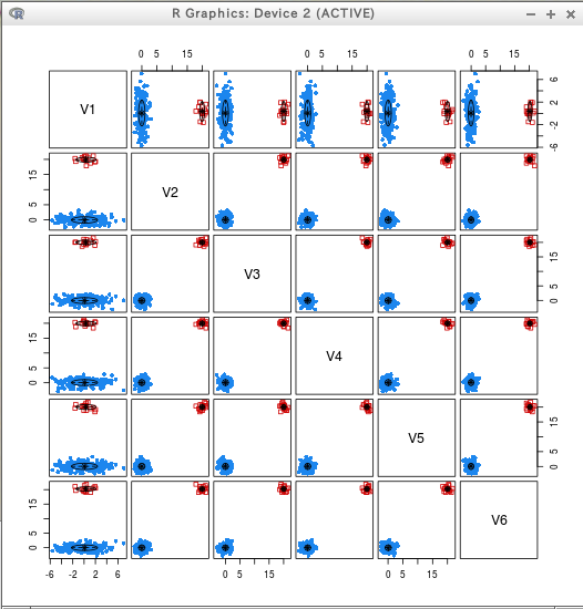
   

   

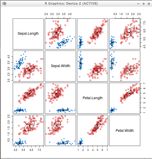
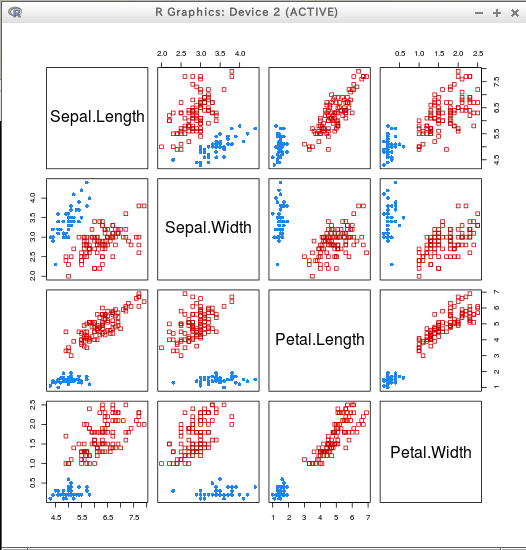
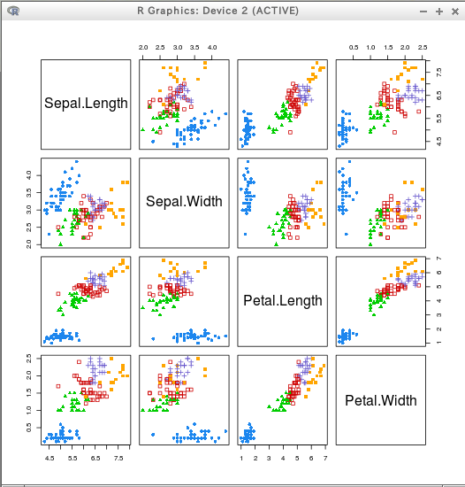
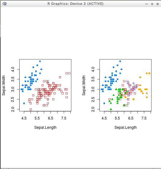
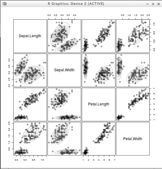
   * iris

   require(mclust)
   C3 = Mclust(iris[,c(1:4)])
   summary(C3)
   plot(C3)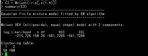
   

   
   
3. クラスタリング結果を整数ベクトルで得る (get clustering result)

   * テストデータ

   C$classification
   C$uncertainty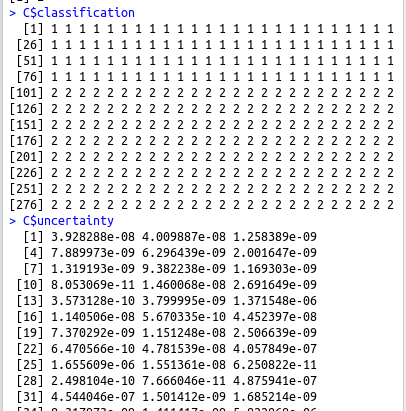
   

   

   C2$classification
   C2$uncertainty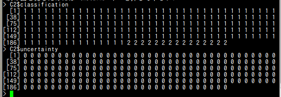
   

   

   * iris

   C3$classification
   C3$uncertainty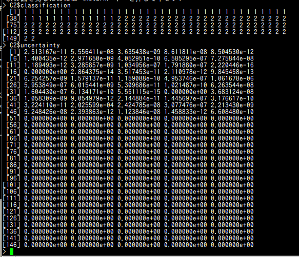
   

   
4. 元データとクラスタに関する属性の表示
   • n : データの観測数 (The number of observations in the data.)
   • d : データの次元 (The dimension of the data.)
   • G : 最適なクラスタ数 (The optimal number of mixture components.)

   * テストデータ

   C$d
   C$n
   C$G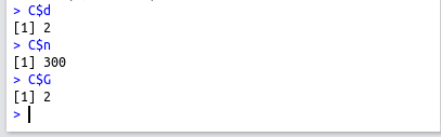
   

   

   C2$d
   C2$n
   C2$G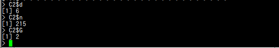
   

   

   * iris

   C3$d
   C3$n
   C3$G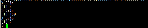
   

   
5. Mclust VVV モデル (ellipsoidal, varying volume, shape, and orientation) model) の各クラスタの属性の表示
   • pro : クラスタの混合率 (A vector whose kth component is the mixing proportion for the kth component of the mixture model. If missing, equal proportions are assumed.)
   • mean : クラスタの平均 (The mean for each component. If there is more than one component, this is a matrix whose kth column is the mean of the kth component of the mixture model.)
   • variance$d : d はデータの次元 (The dimension of the data.)
   • variance$G : G はクラスタ数 (The number of components in the mixture model.)
   • variance$sigma : d かける d かける G の行列. [,,k]はk番目のクラスタの分散共分散行列 (For all multidimensional mixture models. A d by d by G matrix array whose [,,k]th entry is the covariance matrix for the kth component of the mixture model.)
   • variance$cholsigma : d かける d かける G の行列. [,,k]はk番目のクラスタの上三角 Cholesky factor (For the unconstrained covariance mixture model "VVV". A d by d by G matrix array whose [,,k]th entry is the upper triangular Cholesky factor of the covariance matrix for the kth component of the mixture model.)

     * テストデータ

     C$parameters$pro
     C$parameters$mean
     C$parameters$variance$d
     C$parameters$variance$G
     C$parameters$variance$sigma
     C$parameters$variance$cholsigma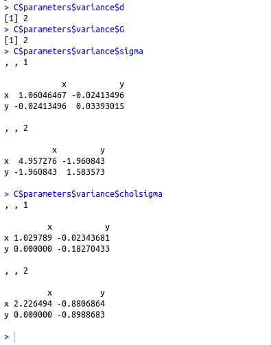
     

     

     C2$parameters$pro
     C2$parameters$mean
     C2$parameters$variance$d
     C2$parameters$variance$G
     C2$parameters$variance$sigma
     C2$parameters$variance$cholsigma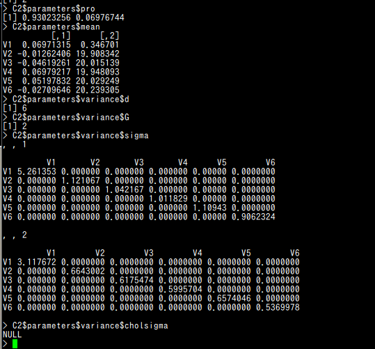
     

     

     * iris

     C3$parameters$pro
     C3$parameters$mean
     C3$parameters$variance$d
     C3$parameters$variance$G
     C3$parameters$variance$sigma
     C3$parameters$variance$cholsigma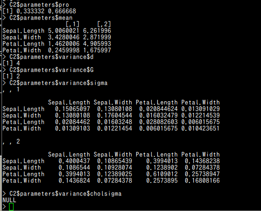
     

     

     確認

     sd(x1)
     sd(y1)
     sd(x2)
     sd(y2)
     sqrt( C$parameters$variance$sigma ) 
     

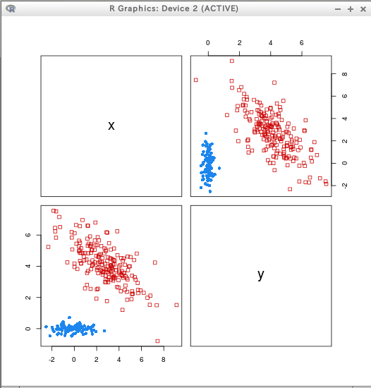
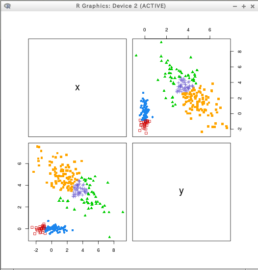
階層クラスタリングと clPairs によるプロット

* テストデータ

hcTree <- hc(modelName = "VVV", data = D)
cl <- hclass(hcTree, c(2,3,4,5))

## 
par(pty = "s", mfrow = c(1,1))
clPairs(D, cl=cl[,"2"])
clPairs(D, cl=cl[,"5"])

hcTree <- hc(modelName = "VVV", data = T)
cl <- hclass(hcTree, c(2,3,4,5))

## 
par(pty = "s", mfrow = c(1,1))
clPairs(T, cl=cl[,"2"])
clPairs(T, cl=cl[,"5"])

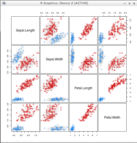
* iris

hcTree <- hc(modelName = "VVV", data = iris[,c(1:4)])
cl <- hclass(hcTree,c(2,3,4,5))

## Not run: 
par(pty = "s", mfrow = c(1,1))
clPairs(iris[,c(1:4)],cl=cl[,"2"])
clPairs(iris[,c(1:4)],cl=cl[,"5"])

階層クラスタリングと coordProj によるプロット

* テストデータ

hcTree <- hc(modelName = "VVV", data = D)
cl <- hclass(hcTree, c(2,3,4,5))

par(mfrow = c(1,2))
dimens <- c(1,2)
coordProj(D, dimens = dimens, classification=cl[,"2"])
coordProj(D, dimens = dimens, classification=cl[,"5"])

hcTree <- hc(modelName = "VVV", data = T)
cl <- hclass(hcTree, c(2,3,4,5))

par(mfrow = c(1,2))
dimens <- c(1,2)
coordProj(T, dimens = dimens, classification=cl[,"2"])
coordProj(T, dimens = dimens, classification=cl[,"5"])

* iris

hcTree <- hc(modelName = "VVV", data = iris[,c(1:4)])
cl <- hclass(hcTree, c(2,3,4,5))

par(mfrow = c(1,2))
dimens <- c(1,2)
coordProj(iris[,c(1:4)], dimens = dimens, classification=cl[,"2"])
coordProj(iris[,c(1:4)], dimens = dimens, classification=cl[,"5"])

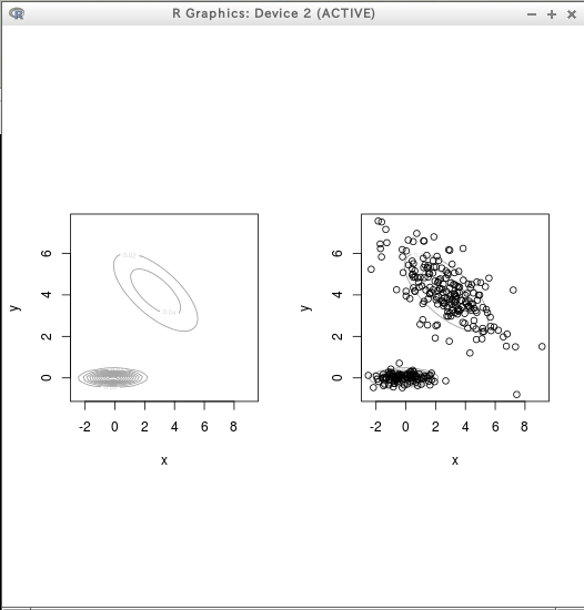
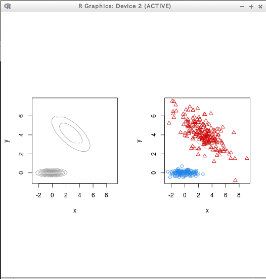
density plot

* テストデータ

require(mclust)
dens = densityMclust(D)
plot(dens)
plot(dens, D)

require(mclust)
dens = densityMclust(T)
plot(dens)
plot(dens, T)

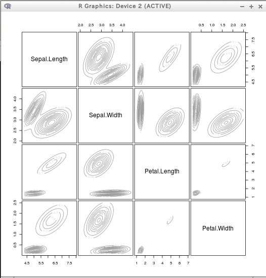
* iris

require(mclust)
dens = densityMclust(iris[,1:4])
plot(dens)
plot(dens, iris[,1:4])

density plot 色付き

* テストデータ

require(mclust)
C = Mclust(D)
dens = densityMclust(D)
plot(dens)
plot(dens, D, col = "grey",
points.col = mclust.options()$classPlotColors[C$classification],
pch = C$classification)

require(mclust)
C2 = Mclust(T)
dens = densityMclust(T)
plot(dens, T, col = "grey",
points.col = mclust.options()$classPlotColors[C2$classification],
pch = C2$classification)

* iris

require(mclust)
C3 = Mclust(iris[,c(1:4)])
dens = densityMclust(iris[,c(1:4)])
plot(dens, iris[,c(1:4)], col = "grey",
points.col = mclust.options()$classPlotColors[C3$classification],
pch = C3$classification)

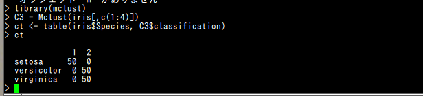
prediction

require(mclust)
C3 = Mclust(iris[,c(1:4)])
ct <- table(iris$Species, C3$classification)
ct