Python のデータフレーム
目次
- オープンデータとソースデータ (data)
- データのバリエーション, 種々の演算 (type)
- ソーシャルビッグデータ基盤, センサネットワークデータベース基盤 (plat)
- データエクスプローラ,Web インタラクションとデータベース (interact)
- 統計基礎、機械学習基礎、画像特徴基礎 (stat)
- 集団行動解析、交通解析、顔の特徴量 (group)
- マイクロアレイの解析 (beppu2)
- 地図データベースの高度応用 (map)
- 一人称型・視点移動画像 (motion)
- 3次元再構成,パノラマ画像,3次元物の特徴量化 (3d)
- 3次元顔 (human face)
オープンデータ (open data) とソースデータ (source data)
オープンデータ (open data)
rdataset.html よりデータを充実。 メタデータの作成。その2点を目指す.
データフレーム
オープンでないソースデータ (source data)
- Image Dataset
-
◆ データ源: http://sourceforge.net/projects/testimages/files/
SAMPLING/, PATTERNS/16BIT/RED_GREEN_BLUE/ などから構成
データのバリエーション, 種々の演算 (type)
段階的に 「オープンデータ の Web ページ」でも公開中
DEM
- shiny を用いた DEM アプリケーションの例
- huagrahuma.dem (topmodel パッケージ) データの紹介 dempyrenees.asc データの紹介
- megdr.html
NASA MEGDR DEM データ
- srtm.htmlShuttle Radar Topography Mission (SRTM) (書きかけ)
- DEM データの操作 (書きかけ)
- mapping DEM data onto RDB.
- 行政区域(面)データ(国土数値情報ダウンロードサービス)
国土数値情報ダウンロードサービス,
行政区域(面)をクリック 国土数値情報(行政区域データ)平成25年度 N03-130401
画像 (image)
OpenData
- http://www.lucnix.be/main.php: Luc Viatour
- http://pixabay.com/ : pixabay
- http://public-domain-photos.com/ : Free Stock Photos
- http://www.picfindr.com/ PicFindr: Free stock photo and image search
距離行列を求め、多次元尺度法で2次元あるいは3次元にマッピングしたとする。 その後、mutiviarate gaussian モデルをあてはめるのは容易である。 次元ののろいがあるかも知れぬ。そこで、距離行列に非線形の関数を当てはめたい。もともと N 次元のランダムな点を 2,3 次元にマッピングするわけである。 このとき、関数を決めるという問題がある.
icp
icp.zip配列 (array)
配列の change point
library(changepoint)
data(Lai2005fig4)
plot(Lai2005fig4[,4])
plot( cpt.mean(Lai2005fig4[,5],method='PELT') )
cpts( cpt.mean(Lai2005fig4[,5],method='PELT') )
時系列 (time series)
配列データ
ftp://ftp.ddbj.nig.ac.jp/ddbj_database/dra/DRA000/DRA000583/DRX001619/
ソーシャルビッグデータ基盤, センサネットワークデータベース基盤 (plat)
計測データ、合成データ、単位、プロファイルの記述体型. 計測日時、計測機器(誤差等)の記述体型. データ探索システムでの処理フローの記録. 合成されたデータの検算・算出プロセスの記録
前提知識
- JSON: DOM シリアライザ,XML と JSON の変換
- リレーショナルデータベース: SQLite 3 と SQLiteman, SQL テーブル定義,SQL 問い合わせ
- Android 開発環境: Android Studio, Android SDK, Android NDK, adb 等のツール
- リレーショナルデータベースの二次索引: create index
- DOT 記法: R の DOT パッケージ
- R のVecStatGraphs2Dパッケージ、RのVecStatGraphs3Dパッケージ
- pca の知識: princomp, pca3d
- ica の知識: R の fastICA パッケージ
データエクスプローラ,Web インタラクションとデータベース (interact)
フォーム、データフロー、Web インタラクション、データの提示における一般性の抽出と、データ記述. 課題の例:
- フォームの形をリレーショナルデータベースに格納.フォームプログラムを動的生成.
- バス停表示のように。縦長形式のダイヤを、横長形式のダイヤに変換したとき、13:10, 13:30 を {10, 30} のように変換する技術
前提知識:
- R, データベース: R, shiny, Redis, Padrino, Sinatra
- shiny (サーバ側) と JavaScript (クライアント側): JQuery でのテーブルエディタ,JQuery でのシリアライズ, JQuery での POST
- リレーショナルデータベース: SQLite 3 と SQLiteman, SQL テーブル定義,SQL 問い合わせ
- Android 開発環境: Android Studio, Android SDK, Android NDK, adb 等のツール
- Androidのインタフェース: Android のタッチインタフェース
- Titanum Mobile Studio and JavaScript, git, node.js
Titanium Mobile Development Environment - Android での Ruby 開発環境: Ruboto を使ってみる(開発環境の設定), Rubotoアプリ製作法, JRuby と Android SDK の連携
- jQuery Mobile
- Web フォーム, テーブル・エディタ,スライダー: JavaScript, JQuery, JQueryUI
- SVG の描画
- DOM シリアライザ:
- URLのリダイレクト
リダイレクトの例 (Sinatra のプログラム)
require 'rubygems'
require 'sinatra'

get %r{^/iris/edit/([0-9]+)$} do
  redirect "http://www.google.co.jp/#q=#{params[:captures]}&safe=off"
end
- Android端末で動くデータベースシステム
キーワード: redis, redis-cli, redis to object mapping
http://memo.saitodev.com/home/arm/arm_cross_compile/, http://absolutearea.blogspot.jp/2012/07/android.html
統計基礎、機械学習基礎、画像特徴基礎 (stat)
統計演算の見える化、統計演算の一貫性と検算.視点移動画像の挙動分析.データエクスプローラ
前提知識:
- R開発環境: Rstudio
- 画像特徴: SIFT, SURF, LBP
- 多次元尺度法: 一般の多次元尺度法,supervised MDS
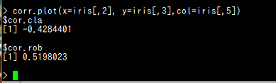
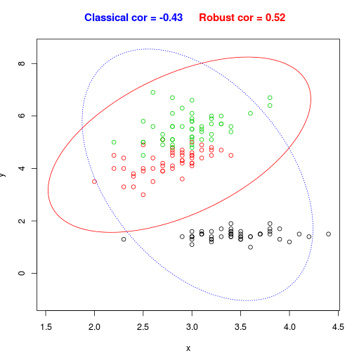
- ガウシアン・モデル: multi viarate gaussian, robust multi viarate gaussian
- 機械学習に関するRパッケージ (gbm, randomForest, party)
- dlib: SURF, HOG, FHOG, Clustering algorithms (linear or kernel k-means, Chinese Whispers, and Newman clustering)
- リレーショナルデータベース: SQLite 3 と SQLiteman, SQL テーブル定義,SQL 問い合わせ
- Android 開発環境: Android Studio, Android SDK, Android NDK, adb 等のツール
- icp の知識: icp.html
- OpenCV の SURF
- OpenCV の Calonder point descriptor (to be done)
- imop
画像フィルタ、イメージ・ピラミッド、ハフ変換、ヒストグラム距離
DOT によるフローの記述
【関連する外部ページ】 http://cran.r-project.org/web/views/Multivariate.html
- meteodate.html
- データエクスプローラシステム
*属性リストをダイナミックに作りたいという課題がある(書きかけ)
- ggplot を用いたグラフ作成
- 時系列予測の R パッケージ
gbm, randomForest - 決定木の R パッケージ
party - machine learning method
https://github.com/zachmayer/rbm
devtools:::install_github('zachmayer/rbm') library(rbm) ?rbm ?rbm_gpu ?stacked_rbm set.seed(10) print('Data from: https://github.com/echen/restricted-boltzmann-machines') Alice <- c('Harry_Potter' = 1, Avatar = 1, 'LOTR3' = 1, Gladiator = 0, Titanic = 0, Glitter = 0) #Big SF/fantasy fan. Bob <- c('Harry_Potter' = 1, Avatar = 0, 'LOTR3' = 1, Gladiator = 0, Titanic = 0, Glitter = 0) #SF/fantasy fan, but doesn't like Avatar. Carol <- c('Harry_Potter' = 1, Avatar = 1, 'LOTR3' = 1, Gladiator = 0, Titanic = 0, Glitter = 0) #Big SF/fantasy fan. David <- c('Harry_Potter' = 0, Avatar = 0, 'LOTR3' = 1, Gladiator = 1, Titanic = 1, Glitter = 0) #Big Oscar winners fan. Eric <- c('Harry_Potter' = 0, Avatar = 0, 'LOTR3' = 1, Gladiator = 1, Titanic = 0, Glitter = 0) #Oscar winners fan, except for Titanic. Fred <- c('Harry_Potter' = 0, Avatar = 0, 'LOTR3' = 1, Gladiator = 1, Titanic = 1, Glitter = 0) #Big Oscar winners fan. dat <- rbind(Alice, Bob, Carol, David, Eric, Fred) #Fit a PCA model and an RBM model PCA <- prcomp(dat, retx=TRUE) RBM <- rbm_gpu(dat, retx=TRUE, num_hidden=2) #Examine the 2 models round(PCA$rotation, 2) #PCA weights round(RBM$rotation, 2) #RBM weights - Restricted-Bolzmann-Machines
darch: Package for deep architectures and Restricted-Bolzmann-Machines
画像特徴
URL: http://www.cse.oulu.fi/CMV/Downloads
see www.cse.oulu.fi facerec image garally
URL: http://www.cs.columbia.edu/CAVE/software/curet/html/download.html
see CUReT
前提知識
キーワード:カメラ式検知器の研究開発、人や商店や駅の集団行動分析.転倒転落、シチュエーション分析、個体識別、交通情報
アンドロイドセンサーアプリ
提供されたサンプルプログラム /home/kkaneko/docs/group/2_06_2014.tar を使用
import 元として Android/sample/BTBoxManagerSample を指定
http://sourceforge.net/projects/dclib/
dlib の画像処理の機能の一部 (Web ページ作成中)
dlib の機械学習の機能の一部 (tobe)
画像処理、機械学習の機能をもったソフトウェア
http://sourceforge.net/projects/scene/files/?source=navbar
前提知識
インストール手順
◆ Ubuntu でのビルド手順例
情報源
D. G. Lowe. Distinctive image features from scale-invariantkeypoints.
International Journal of Computer Vision (IJCV), 60(2):91-110, 2004.
Y. Ke and R. Sukthankar. PCA-SIFT: A More Distinctive
Representation for Local Image Descriptors. 2004.
URL: http://www.asl.ethz.ch/people/lestefan/personal/BRISK
see BRISK
H. Bay, A. Ess, T. Tuytelaars, and L. V. Gool. SURF:
Speeded up robust features. Computer Vision and Image Un-
derstanding (CVIU), 110(3):346-359, 2008.
https://docs.opencv.org/doc/tutorials/features2d/feature_homography/feature_homography.html
屋内全域の再構成、平面成分の分析、法線ベクトルのクラスタリング、色とテクスチャの分析
必要となる知識
【関連する外部ページ】
https://docs.opencv.org/trunk/modules/contrib/doc/facerec/
Point Cloud Rendering
http://opencv.jp/opencv2-x-samples/point-cloud-rendering
情報源
http://sourceforge.net/projects/openbio/
Visual C++ でコンパイルできる
プログラムなど
install a LBP package on Octave system
see: od/data/att_faces.tar.Z
http://www.cl.cam.ac.uk/research/dtg/attarchive/facedatabase.html
点の分布をN次元の正規分布で表現.正規分布の主軸をN個求めることを行いたい.
keywords: mclust, density plot
mvoutlier packages
前準備として facerec の knn.m などを準備しておく
to be filled
to be filled
SVD using OpenCV
Matrix3d P = Matrix3d::Random(3, 3);
JacobiSVD svd(P, Eigen::ComputeFullU | Eigen::ComputeFullV);
MatrixXd S = svd.singularValues();
Matrix3d U = svd.matrixU();
Matrix3d V = svd.matrixV();
cascade classifier
https://docs.opencv.org/doc/tutorials/objdetect/cascade_classifier/cascade_classifier.html#cascade-classifier
rubust pca
robust pca sample
image histogram
グラフ作成
この Web ページで行うこと: プログラムによるグラフ作成
key word: libpcl, in-hand 3d scanner, data capture
asc to off converter
http://www.archeos.eu/wiki/doku.php/
http://www.blensor.org/
# python3.3
sudo apt-get install python-software-properties
sudo add-apt-repository ppa:fkrull/deadsnakes
sudo apt-get update
sudo apt-get install python3.3
sudo apt-get install python3.3-dev
wget https://bitbucket.org/pypa/setuptools/raw/bootstrap/ez_setup.py
sudo python3.3 ez_setup.py
git clone https://github.com/mgschwan/blensor.git
cd blensor
mkdir a
cd a
cmake -DWITH_PYTHON=OFF -DPYTHON_VERSION=3.3m PYTHON_INCLUDE_DIR=/usr/include/python3.3m -DWITH_OPENIMAGEIO=OFF -DWITH_IMAGE_OPENJPEG=OFF -DWITH_OPENAL=OFF -DWITH_SPACENAV=OFF -DWITH_CYCLES=OFF -DWITH_SYSTEM_GLEW=OFF -DWIGH_GPU=OFF ..
some features
BSS-1 implementation of a Kinect Sensor
Support to obtain accurate depth map information
Support the output to the PCD format from the PCL (Point cloud library)
Starting with version 1.0.10 the RGB values of the material are stored in the PCD and EVD file
Tutorial for PCL developers/users
Render a pointcloud in blender
http://graphics.stanford.edu/data/3Dscanrep/
https://d.hatena.ne.jp/etopirika5/20101027/1288152036
Cloud Compare, admesh, stl オープンソースソフトウェア
* データ源の URL: http://sourceforge.net/projects/mecab/files/
連続する2フレームから keypoint の時間特徴量をとりだす。
さらに、離れたフレームの列から大域的な情報を出す(x, y, size, angle 等の時間変化になる)。
これで分析を行う。
集団行動解析、交通解析 (group)
BT タグ・アプリ (BT tag)
findViewById の DeviceListActivity, FilteredDeviceListActivity の部分を削除
背景除去と動体検知 (background subtraction and object tracking) (group)
cd /tmp
tar -xvjof dlib-18.7.tar.bz2
cd dlib-18.7
cd examples
cmake .
sed -i 's/-llapack/-llapack -L\/usr\/lib\/atlas-base -latlas/' CMakeFiles/*.txt CMakeFiles/*/*.txt
cmake --build . --config Release
Face_Detection
FHOG_Feature_Extraction
FHOG_Object_Detection
Image
SURF
Object_Detector
Object_Detector_Advanced
Train_Object_Detector
Graph_Labeling
Unsupervised
cca
empirical_kernel_map
kcentroid
linearly_independent_subset_finder
sammon_projection
svm_one_class_trainer
vector_normalizer
vector_normalizer_pca
Kernel_Centroid
Kernel_K-Means_Clustering
Kernel_Ridge_Regression
Kernel_RLS_Filtering
Kernel_RLS_Regression
KRR_Classification
Linear_Manifold_Regularizer
Multiclass_Classification
cd /tmp
sudo dkpg -i  Scene-1.0.3-i386.deb
地図データベースの高度応用 (map)
source("http://bioconductor.org/biocLite.R")
biocLite("hypergraph")
biocLite("RBGL")
biocLite("GraphPart")
biocLite("Rgraphviz")
# to turn the snacoreex.gxl (from RBGL package) graph to a hypergraph
# this is a rough example
kc_hg_n <- c("A", "C", "B", "E", "F", "D", "G", "H", "J", "K", "I", "L", "M", "N", "O", "P", "Q", "R", "S", "T", "U")
kc_hg_e <- list(c("A", "C"), c("B", "C"), c("C", "E"), c("C", "F"), c("E", "D"), c("E", "F"), c("D", "G"), c("D", "H"), c("D", "J"), c("H", "G"), c("H", "J"), c("G", "J"), c("J", "M"), c("J", "K"), c("M", "K"), c("M", "O"), c("M", "N"), c("K", "N"), c("K", "F"), c("K", "I"), c("K", "L"), c("F", "I"), c("I", "L"), c("F", "L"), c("P", "Q"), c("Q", "R"), c("Q", "S"), c("R", "T"), c("S", "T"))
kc_hg_he <- lapply(kc_hg_e, "Hyperedge")
kc_hg <- new("Hypergraph", nodes=kc_hg_n, hyperedges=kc_hg_he)
plot(
kCoresHypergraph(kc_hg)
一人称型・視点移動画像 (motion)
コーナー
コーナー検出(EigenValue,Harris,FAST) | OpenCV.jp
http://opencv.jp/opencv2-x-samples/corner_detection
keypoints
cd /tmp
unzip OpenSURFcpp.zip
applications using keypoints
3次元再構成,パノラマ画像,3次元物の特徴量化 (3d)
3次元顔 (human face)
G. B. Huang, M. Ramesh, T. Berg, and E. Learned-miller. Labeled
faces in the wild: A database for studying face recognition in un-
constrained environments. In ECCV Workshop on Faces in Real-life
Images, 2008
L. Wolf, T. Hassner, and I. Maoz. Face recognition in unconstrained
videos with matched background similarity. In CVPR, 2011.
sudo add-apt-repository ppa:v-launchpad-jochen-sprickerhof-de/pcl
sudo apt-get update
sudo apt-get install libpcl-all
Filter points based on their local point densities. Remove points
that are sparse relative to the mean point density of the whole
cloud.
filtering.cpp
pcl::StatisticalOutlierRemoval
void
detectkeypoints(pcl::PointCloud
void
PFHfeaturesatkeypoints(pcl::PointCloud
keypoints.cpp
void
featurecorrespondences(pcl::PointCloud
#include
#include
#include
#!/bin/bash
# 64x96 サイズの pgm 画像生成
cd /home/kkaneko/rinkou/od/data/ColorFERETDatabase/colorferet/dvd2/data/images/00740
cp *.bz2 /tmp
cd /tmp
bzip2 -d *.ppm.bz2
for i in *.ppm; do
  echo $i
  convert -resize 64x96 $i `basename $i .ppm`.pgm
done
http://libface.sourceforge.net/file/Download.html
cmake -DBUILD_EXAMPLES_GUI=1 -DBUILD_EXAMPLES=1 .
g++ -I/usr/local/include -o FaceDetection FaceDetection.cpp -L/usr/local/lib -lface -lhighgui -lcv -lcxcore -lcvaux
数値ベクトルの集合 (a set of numeric vectors)

ベクトルの classifier (classifier)
    k-Nearest Neighbor; available distance metrics
        Euclidean Distance
        Cosine Distance
        ChiSquare Distance
        Bin Ratio Distance
P=[1,21,20,2,4,30; 1,21,20,2,4,30]
y=[1, 3, 3, 2, 2, 3]
Q=[1;1]

% returns 1
knn(P,y,Q,1)
% returns 2
knn(P,y,Q,3)
% returns 3
knn(P,y,Q,6)
Point Cloud
require "csv"
# 行数カウント
lines=0
reader = CSV.open("/tmp/Sinus_pts.asc", "r")
reader.each do |row|
  lines = lines + 1
end
reader.close
# 出力
print "OFF\n"
print "#{lines} 0 0 \n"
reader = CSV.open("/tmp/Sinus_pts.asc", "r")
reader.each do |row|
  print "#{row[0]} #{row[1]} #{row[2]}\n"
end
reader.close
Computer Vision and Geometry Group
https://www.google.co.jp/url?sa=t&rct=j&q=&esrc=s&source=web&cd=1&sqi=2&ved=0CCsQFjAA&url=http%3A%2F%2Fwww.cvg.ethz.ch%2Fteaching%2F2012spring%2F3dphoto%2FSlides%2F3dphoto_pcl_tutorial.pdf&ei=M1B0UoSrLof3lAX3s4EQ&usg=AFQjCNHg0Zje3kCIxP2c7PucrMDg_ndarg&sig2=sEKO4QmbX0XJI5eFO-Gupg&bvm=bv.55819444,d.dGI
unzip data_capture.zip
'cmake ../data_capture' and then execute 'make'.
3次元地図
PCL / STL / PLY
辞書
* bio の例(normalize を例題に)
* R のパッケージ
https://github.com/ajdamico/usgsd/blob/master/National%20Health%20Interview%20Survey/download%20all%20microdata.R
usgsd / National Health Interview Survey / download all microdata.R
library(rgl)
---
library(rgl)
open3d()
x <- sort(rnorm(1000))
y <- rnorm(1000)
z <- rnorm(1000) + atan2(x,y)
plot3d(x, y, z, col=rainbow(1000))
---
points3d(x, y = NULL, z = NULL, ...)
lines3d(x, y = NULL, z = NULL, ...)
segments3d(x, y = NULL, z = NULL, ...)
triangles3d(x, y = NULL, z = NULL, ...)
quads3d(x, y = NULL, z = NULL, ...)
---
library(foreign)
---
library(foreign)
read.spss()
write.foreign( "SPSS" )
library(misc3d)
---
library(misc3d)
contour3d(...)
kde3d(...)
d <- kde3d(quakes$long, quakes$lat, quakes$depth, n = 40)
contour3d(d$d, exp(-12), d$x/22, d$y/28, d$z/640,
color = "green", color2 = "gray", scale=FALSE,
engine = "standard")
plot3d(quakes$lat, quakes$long, quakes$depth, col=rainbow(1000))
---
-----
terasvirta test
library(tseries)
x <- runif(1000, -1, 1)
y <- x^2 - x^3 + 0.1*rnorm(x)
plot(x,y)
terasvirta.test(x, y)
terasvirta.test(cbind(x,x^2,x^3), y)
x[1] <- 1.0
for(i in (2:n)) {
x[i] <- 0.98*x[i-1] + 0.01
}
x <- as.ts(x)
plot(x)
terasvirta.test(x)
terasvirta.test(cbind(x,x^2,x^3))
help.zelig("models")
https://www.google.com/url?sa=t&rct=j&q=&esrc=s&source=web&cd=4&cad=rja&ved=0CE0QFjAD&url=http%3A%2F%2Fwww.slideshare.net%2Fizahn%2Frstatistics&ei=S3DyUYPPIcKnkAXA1YGACg&usg=AFQjCNF_FBDkMjpj7vEC-nJ17igMYTmKaQ&sig2=CjWahfa1dXy-O3hLWffgTg
http://cran.r-project.org/web/views/TimeSeries.html
library( forecast )
tsdisplay( LakeHuron )
data1 <- auto.arima( LakeHuron )
plot( forecast( data1, h=10 ) )
現在あるいは直近の測定値に加えて、
過去の測定値の集積から、統計的手法などを用いて、直近の測定値と現在時刻の時間のずれの補償や、
測定漏れの補間や、将来の予測を行うとする.
たとえば、
ありえる事象の集合である母集団の個々の観測値を表す確率変数Xについて、
Xが正規分布に従うことが前もって分かっていたり、
母集団の観測の集積から、Xが正規分布の従うということがある確からしさで言えるとする。
確率モデルから、観測値あるいは観測値の時系列集合を自動的に生成できるし、
観測値の集積から確率モデルを導くことができる。
この両方向の処理を繰り返しても、確率モデルが変化しないとき、この確率モデルは安心して使うことができる。
Xが time-variable (時系列変数)であるとき、
この場合、
ずれの補償:
補間:
将来の予測:
過去の測定値の集計から、ある時刻tでの値を予測し、これを実測値にあてはめることで、予測の良さを評価することもできる。
<要因とランダム性>
要因のランダム性によって、ある変数Yの値が変化するとする.要因Xがランダム変数であり、要因YがXの積分値とすると、Yは典型的なランダムウオークである.
このときYの統計モデルではなく、要因の統計モデルが作られる
要因の統計モデルと観測値
派生変数の観測値、
<要因の予測とランダム性>
要因がランダムであるというからには、予測はしがたい.
単に「平均E,分散sの正規分布で値集合を合成し、その中から、ランダムに選ぶ」ということになる(モンテカルロシミュレーションのような状況になる.
予測と言っているのは、無限区間での一様分布(まったくの無知識)よりも、統計モデルがあったほうが、現実に近い要因知を合成できると言っているに過ぎない。
要因をすべて無視して、「速度」は正規分布であるという仮説を立てることもできる。
(要因なし。派生変数を直接、統計モデル化)
ある要因を入れることで、精度がAだけ向上する確率(精度の尺度は別途定義する)はPだということができるようになる.例えば混合ガウス分布。この場合には、要因は確率変数だが、派生変数は、要因に従属する変数である。
要因、派生変数ともに観測可能な値であるとする。
3章
では、
・緯度経度のプロット
・バス停の到着と発車はわかる
・バス停の到着と発車の集積もある
このとき、
要因と派生変数の関連の仮設を立て、
派生変数の観測値から、要因の統計モデルと観測値を作りたいとする.
要因
曜日区分:平日、土曜・日曜・祝日、土曜、日曜、祝日、三連休、年末年始、お盆
天候
時間帯
未知の突発行事
始点の出発時刻。始点の乗客数はある確度で言える。
観測される派生変数は、
各バス停における到着時刻と乗客数である.
将来、各バス停における到着時刻、各バス停における乗客数、現在位置、現在速度を推定したい。(例えば、信頼区間やp値を使って)
<検定>
時系列の変数Yの任意の時刻の観測値Y(t)を、t以前の値から推定し、観測値との差の平均の差、標準偏差、尖度、歪度を求める
さまざまな表示法
<地図での、あなたはここです。バスはここです。お探しの場所はここです表示>
<地図での、バスに固有の表示法>
<バス時刻表だが。。。>
10 | 10 30 50
10 | 14 33 50-54
下段は過去の実績だったり、予測値だったりする。
予測値の区間 [l, u]について、lの値は、100%どんなことがあっても、これより早くは来ない。という意味になる。
l は、いまのバスまでの走行距離/法定速度、あるいは、過去の実績の最高速度
<いまは混んでいるのか、空いているのかの予測表示>
状態そのものの表示
先行するバスがあると、後ろのバスは早いという現象
ビデオ素材 (video)