VBGMM (Variational Bayesian Gaussian Mixture) を用いてクラスタリング（Python, scikit-learn を使用）

前準備

Python の準備（Windows，Ubuntu 上）

• Windows での Python 3.10，関連パッケージ，Python 開発環境のインストール（winget を使用しないインストール）: 別ページ »で説明
• Ubuntu では，システム Pythonを使うことができる．Python3 開発用ファイル，pip, setuptools のインストール: 別ページ »で説明

【サイト内の関連ページ】

• Python のまとめ: 別ページ »にまとめ
• Google Colaboratory の使い方など: 別ページ »で説明

【関連する外部ページ】 Python の公式ページ: https://www.python.org/

Python の numpy, pandas, seaborn, matplotlib, scikit-learn のインストール

• Windows の場合

  Windows では，コマンドプロンプトを管理者として実行し， 次のコマンドを実行する．

  python -m pip install -U pip setuptools numpy pandas matplotlib seaborn scikit-learn scikit-learn-intelex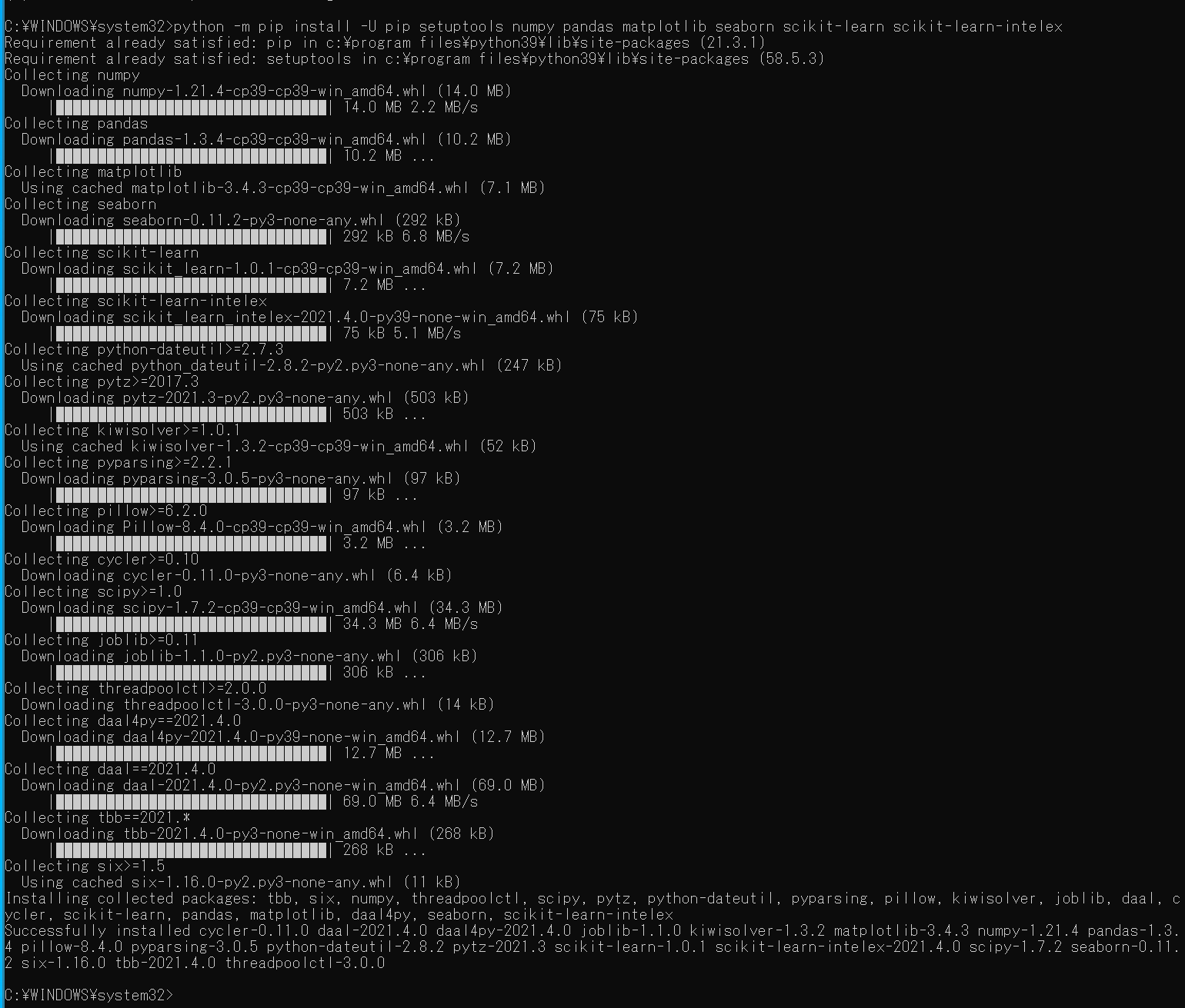
  

  
• Ubuntu の場合

  端末で，次のコマンドを実行

  sudo apt -y update
  sudo apt -y install python3-numpy python3-pandas python3-seaborn python3-matplotlib python3-sklearn
  

3. Iris データセットの準備

1. Iris データセットの読み込み

   import pandas as pd
   import seaborn as sns
   sns.set()
   iris = sns.load_dataset('iris')
   

2. データの確認

   print(iris.head())
   

3. 形と次元を確認

   配列（アレイ）の形： サイズは 150 ×5．次元数は 2． 最後の列は，iris.target は花の種類のデータである

   print(iris.shape)
   print(iris.ndim)
   

4. Iris データセットの0, 1, 2, 3列目を表示

   print( iris.iloc[:,0:4] )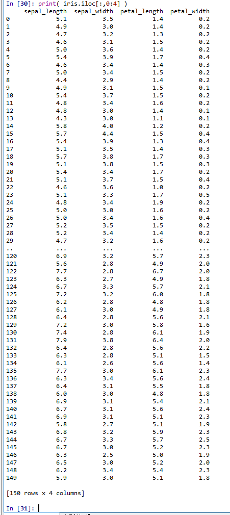
   

   

VBGMM (Variational Bayesian Gaussian Mixture) によるクラスタリング

1. 散布図に主成分分析プロットの準備

   # 主成分分析
   def prin(A, n):
       pca = sklearn.decomposition.PCA(n_components=n)
       return pca.fit_transform(A)
   
   # 主成分分析で２つの成分を得る
   def prin2(A):
       return prin(A, 2)
   
   # M の最初の2列を，b で色を付けてプロット．b はラベル
   def scatter_label_plot(M, b, alpha):
       a12 = pd.DataFrame( M[:,0:2], columns=['a1', 'a2'] )
       f = pd.factorize(b)
       a12['target'] = f[0]
       g = sns.scatterplot(x='a1', y='a2', hue='target', data=a12, palette=sns.color_palette("hls", np.max(f[0]) + 1), legend="full", alpha=alpha)
       # lenend を書き換え
       labels=f[1]
       for i, label in enumerate(labels):
           g.legend_.get_texts()[i].set_text(label) 
       plt.show()
   
   # 主成分分析プロット
   def pcaplot(A, b, alpha):
       scatter_label_plot(prin2(A), b, alpha)
   

2. Iris データセットの0, 1, 2, 3列目について、VBGMM (Variational Bayesian Gaussian Mixture) を用いてクラスタリング

   import numpy as np
   from sklearn.mixture import BayesianGaussianMixture
   
   bgmm = BayesianGaussianMixture(n_components=10, verbose=1).fit(iris.iloc[:,0:4]) 
   X = iris.iloc[:,0:4].values
   c = bgmm.predict(X)
   print(c)
   

3. 結果をプロット

   乱数を使っているので、実行するたびに違った値になる

   pcaplot(X, c, 1)   
   

4. 比較のため，Iris データセットをプロット

   pcaplot(X, iris.iloc[:,4], 1)