huagrahuma.dem (topmodel パッケージ) データの紹介
前準備
使用するソフトウェア
- R システムのインストールが済んでいること
huagrahuma, huagrahuma.dem データセット
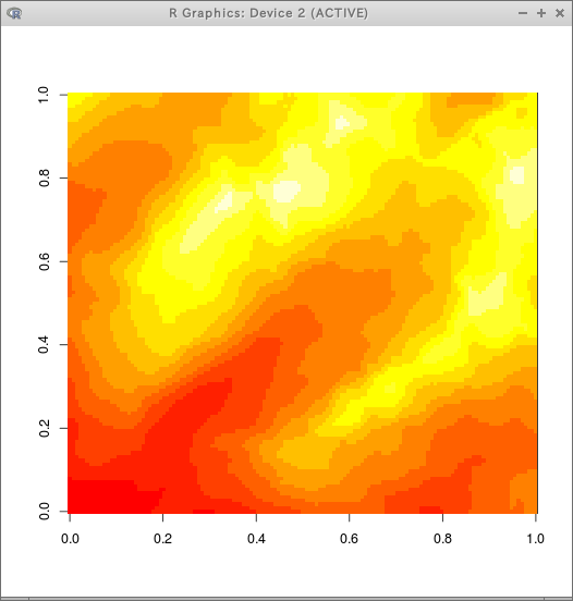
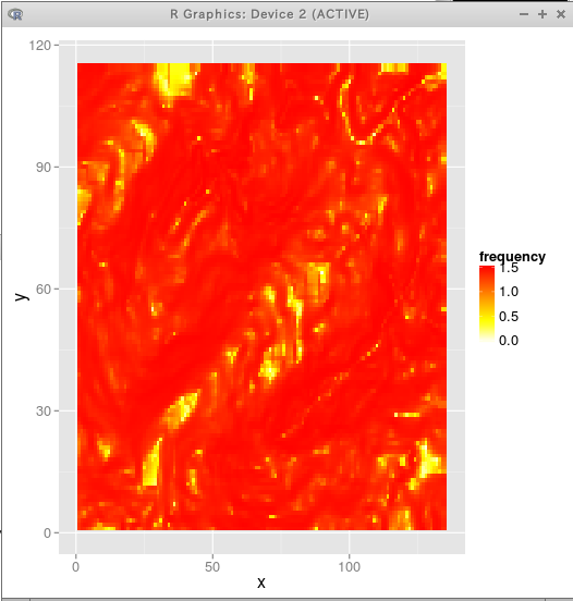
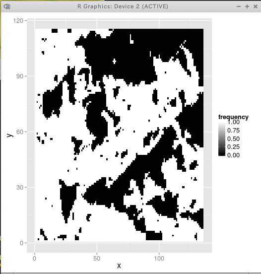
image 関数による表示 (例)
require(topmodel)

data(huagrahuma)
data(huagrahuma.dem)

image(huagrahuma.dem)
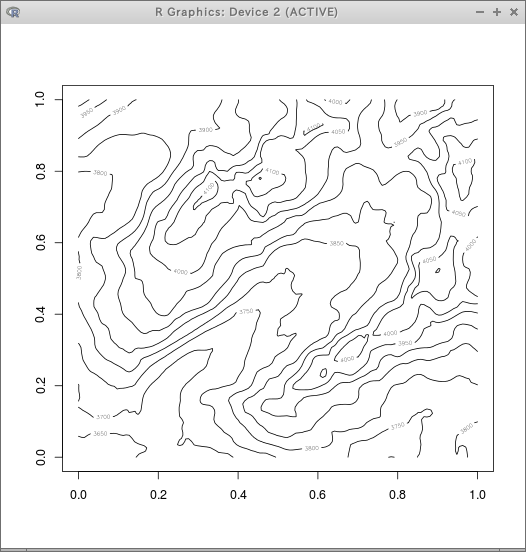
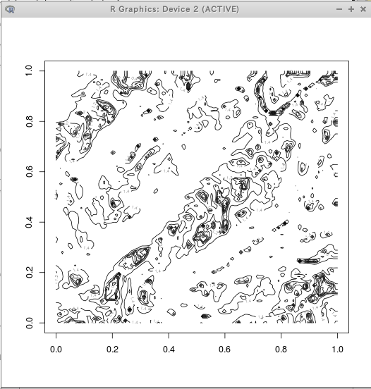
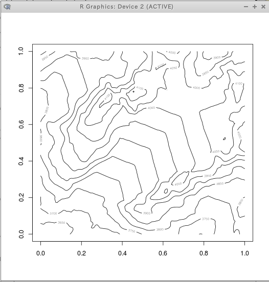
contour 関数による表示 (例)
require(topmodel)
data(huagrahuma)
data(huagrahuma.dem)
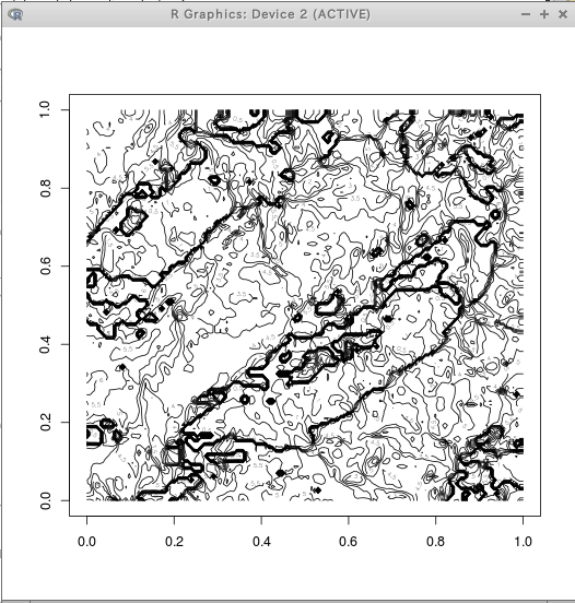
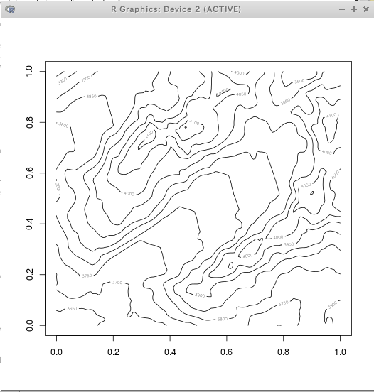
contour(huagrahuma.dem)
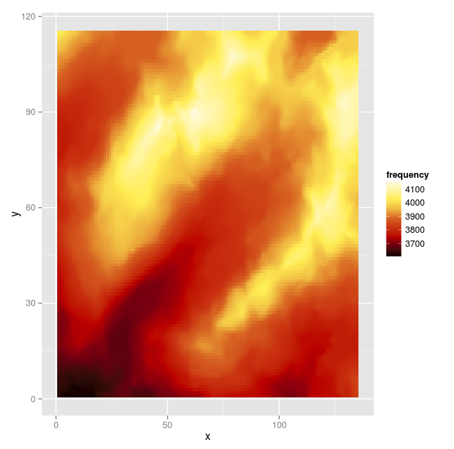
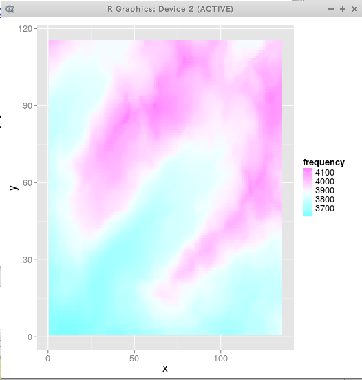
ggplot 関数を用いた表示 (例)
【関連する外部ページ】 http://zoas.blog112.fc2.com/blog-entry-1.html
require(ggplot2)
require(topmodel)
require(data.table)
data(huagrahuma)
data(huagrahuma.dem)
plotdem <- function(DEM, c) {
x <- rep(1:nrow(DEM), ncol(DEM)) # 1 2 3 1 2 3 1 2 3 1 2 3
y <- rep(1:ncol(DEM), each=nrow(DEM)) # 1 1 1 1 2 2 2 2 3 3 3 3
T <- data.table(x=x, y=y, val=as.numeric(DEM))
ggplot(T, aes(x=x, y=y, fill=val)) + geom_tile() + scale_fill_gradientn("frequency", colours = c)
}
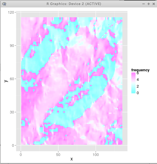
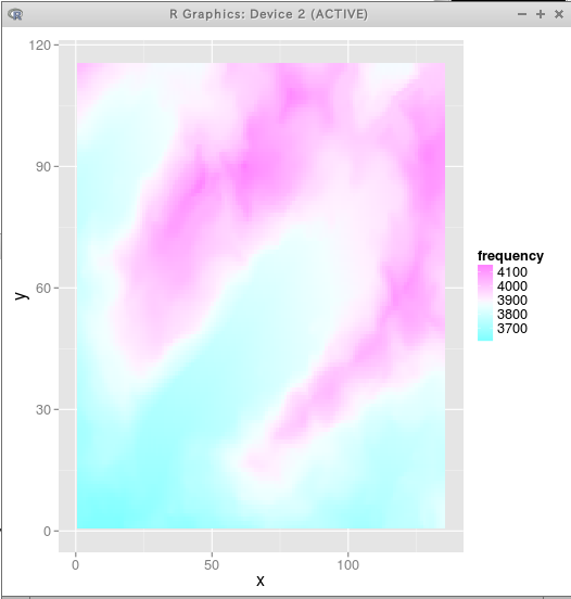
plotdem(huagrahuma.dem, cm.colors(20))
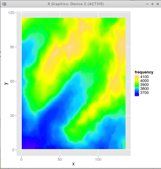
plotdem(huagrahuma.dem, topo.colors(20))
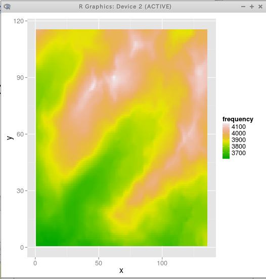
plotdem(huagrahuma.dem, terrain.colors(20))
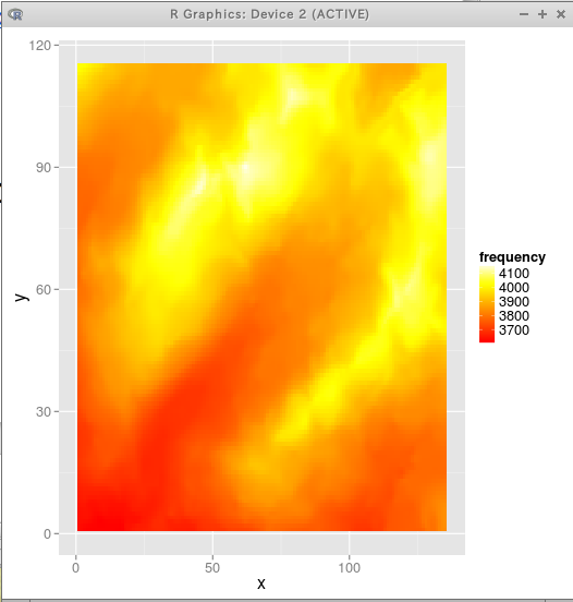
plotdem(huagrahuma.dem, heat.colors(20))
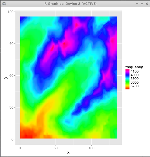
plotdem(huagrahuma.dem, rainbow(20))
◆ plotdem(huagrahuma.dem, cm.colors(20))
◆ plotdem(huagrahuma.dem, topo.colors(20))
◆ plotdem(huagrahuma.dem, terrain.colors(20))
◆ plotdem(huagrahuma.dem, heat.colors(20))
◆ plotdem(huagrahuma.dem, rainbow(20))
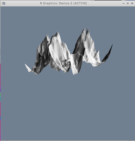
persp 関数による表示 (例)
require(topmodel)

data(huagrahuma)
data(huagrahuma.dem)

persp(huagrahuma.dem, theta = 135, phi = 30, shade=0.75, border=NA, box=FALSE )
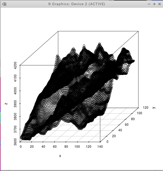
scatterplot3d 関数による表示 (例)
require(scatterplot3d)
require(topmodel)

data(huagrahuma)
data(huagrahuma.dem)


rgldem <- function(DEM, col) {
  x <- rep(1:nrow(DEM), ncol(DEM))      # 1 2 3 1 2 3 1 2 3 1 2 3
  y <- rep(1:ncol(DEM), each=nrow(DEM)) # 1 1 1 1 2 2 2 2 3 3 3 3
  z <- as.numeric(DEM)
  scatterplot3d( x, y, z )
}

rgldem(huagrahuma.dem)
勾配強度
insol パッケージの cgrad + slope
require(ggplot2)
require(topmodel)
require(insol)
require(data.table)
data(huagrahuma)
data(huagrahuma.dem)
plotdem <- function(DEM, c) {
x <- rep(1:nrow(DEM), ncol(DEM)) # 1 2 3 1 2 3 1 2 3 1 2 3
y <- rep(1:ncol(DEM), each=nrow(DEM)) # 1 1 1 1 2 2 2 2 3 3 3 3
T <- data.table(x=x, y=y, val=as.numeric(DEM))
ggplot(T, aes(x=x, y=y, fill=val)) + geom_tile() + scale_fill_gradientn("frequency", colours = c)
}
slopedem <- function(DEM, dl_long, dl_lat) {
return( slope( cgrad(DEM, dl_long, dl_lat) ) )
}
plotdem(slopedem(huagrahuma.dem, 1, 1), rev(heat.colors(20)))
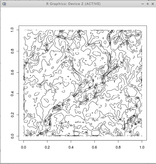
contour(slopedem(huagrahuma.dem, 1, 1))
◆ plotdem(slopedem(huagrahuma.dem, 1, 1), rev(heat.colors(20)))
◆ contour(slopedem(huagrahuma.dem, 1, 1))
斜面の向き
insol パッケージの cgrad + aspect
require(ggplot2)
require(topmodel)
require(insol)
require(data.table)

data(huagrahuma)
data(huagrahuma.dem)


plotdem <- function(DEM, c) {
  x <- rep(1:nrow(DEM), ncol(DEM))      # 1 2 3 1 2 3 1 2 3 1 2 3
  y <- rep(1:ncol(DEM), each=nrow(DEM)) # 1 1 1 1 2 2 2 2 3 3 3 3

  T <- data.table(x=x, y=y, val=as.numeric(DEM))
  ggplot(T, aes(x=x, y=y, fill=val)) + geom_tile() + scale_fill_gradientn("frequency", colours = c)
}


aspectdem <- function(DEM, dl_long, dl_lat) {
  return( aspect( cgrad(DEM, dl_long, dl_lat) ) )
}

plotdem(aspectdem(huagrahuma.dem, 1, 1), cm.colors(20))
contour(aspectdem(huagrahuma.dem, 1, 1))
◆ plotdem(aspectdem(huagrahuma.dem, 1, 1), cm.colors(20))
◆ contour(aspectdem(huagrahuma.dem, 1, 1))
topmodel パッケージの sinkfill
require(ggplot2)
require(topmodel)
require(insol)
require(data.table)

data(huagrahuma)
data(huagrahuma.dem)


plotdem <- function(DEM, c) {
  x <- rep(1:nrow(DEM), ncol(DEM))      # 1 2 3 1 2 3 1 2 3 1 2 3
  y <- rep(1:ncol(DEM), each=nrow(DEM)) # 1 1 1 1 2 2 2 2 3 3 3 3

  T <- data.table(x=x, y=y, val=as.numeric(DEM))
  ggplot(T, aes(x=x, y=y, fill=val)) + geom_tile() + scale_fill_gradientn("frequency", colours = c)
}

plotdem( sinkfill(huagrahuma.dem, 25, 5), cm.colors(20) )
contour(sinkfill(huagrahuma.dem, 25, 5))
plotdem( sinkfill(huagrahuma.dem, 25, 8), cm.colors(20) )
contour(sinkfill(huagrahuma.dem, 25, 8))
◆ plotdem( sinkfill(huagrahuma.dem, 25, 5), cm.colors(20) )
◆ contour(sinkfill(huagrahuma.dem, 25, 5))
◆ plotdem( sinkfill(huagrahuma.dem, 25, 8), cm.colors(20) )
◆ contour(sinkfill(huagrahuma.dem, 25, 8))
topmodel パッケージの topidx
require(ggplot2)
require(topmodel)
require(insol)
require(data.table)

data(huagrahuma)
data(huagrahuma.dem)


plotdem <- function(DEM, c) {
  x <- rep(1:nrow(DEM), ncol(DEM))      # 1 2 3 1 2 3 1 2 3 1 2 3
  y <- rep(1:ncol(DEM), each=nrow(DEM)) # 1 1 1 1 2 2 2 2 3 3 3 3

  T <- data.table(x=x, y=y, val=as.numeric(DEM))
  ggplot(T, aes(x=x, y=y, fill=val)) + geom_tile() + scale_fill_gradientn("frequency", colours = c)
}

plotdem( topidx(huagrahuma.dem, resolution= 25)$atb, rev(heat.colors(20)) )
contour( topidx(huagrahuma.dem, resolution= 25)$atb )
◆ plotdem( topidx(huagrahuma.dem, resolution= 25)$atb, rev(heat.colors(20)) )
◆ contour( topidx(huagrahuma.dem, resolution= 25)$atb )
日照
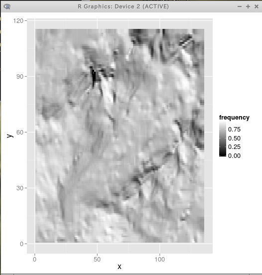
doshade() 関数で影を求める
require(ggplot2)
require(topmodel)
require(insol)
require(data.table)

data(huagrahuma)
data(huagrahuma.dem)


plotdem <- function(DEM, c) {
  x <- rep(1:nrow(DEM), ncol(DEM))      # 1 2 3 1 2 3 1 2 3 1 2 3
  y <- rep(1:ncol(DEM), each=nrow(DEM)) # 1 1 1 1 2 2 2 2 3 3 3 3

  T <- data.table(x=x, y=y, val=as.numeric(DEM))
  ggplot(T, aes(x=x, y=y, fill=val)) + geom_tile() + scale_fill_gradientn("frequency", colours = c)
}


cellsize=header[5,2]
sv=normalvector(65,315)
sh=doshade(huagrahuma.dem, sv, 1)

plotdem(sh, grey(1:100/100))
関数化の途中
## add intensity of illumination in this case sun at NW 45 degrees elevation
sv=normalvector(45, 315)
grd=cgrad(huagrahuma.dem, cellsize)
hsh=grd[,,1]*sv[1]+grd[,,2]*sv[2]+grd[,,3]*sv[3]
## remove negative incidence angles (self shading)
hsh=(hsh+abs(hsh))/2
sh=doshade(huagrahuma.dem, sv, cellsize)
plotdem(hsh*sh, grey(1:100/100))
insol パッケージに日陰、日当たりの機能あり
M <- array( c( x, y, D ), dim=c(nrow(D), ncol(D), 3) );