VBGMM (Variational Bayesian Gaussian Mixture) を用いてクラスタリング(Python, scikit-learn を使用)
【概要】
VBGMM (Variational Bayesian Gaussian Mixture) では,クラスタ数を指定せずにクラスタリングを行う.本記事では,Python と scikit-learn を使用し,Iris データセットに VBGMM を適用する.VBGMM は,あらかじめ与えた最大クラスタ数のうち,データに適合するクラスタにだけ大きな重みを割り当て,有効なクラスタ数を自動的に決定する(実際に使われないクラスタの重みは 0 に近い値になる).クラスタリング結果は主成分分析(PCA:データの分散が大きい方向に軸を取り直して次元を減らす手法)で2次元に次元削減し,散布図として可視化する.元の Iris データセットの品種ラベルによるプロットと比較することで,分類のようすを視覚的に確認できる.
【目次】
- 1. Python 3.12 のインストール
- 2. Python の開発環境 Visual Studio Code のインストールと Python 用の設定
- 3. Python プログラム実行手順
- 4. 必要なライブラリのインストール
- 5. 実行のための準備とその確認手順(Windows 前提)
- 6. 概要・使い方・実行上の注意
- 7. 演習:VBGMM による Iris データのクラスタリングと可視化
- 8. まとめ
【関連する外部ページ】
【サイト内の関連情報】
1. Python 3.12 のインストール
2. Python の開発環境 Visual Studio Code のインストールと Python 用の設定
3. Python プログラム実行手順
4. 必要なライブラリのインストール
管理者権限でコマンドプロンプトを起動する
(手順:Windowsキーまたはスタートメニュー → cmd と入力 → 右クリック → 「管理者として実行」)。
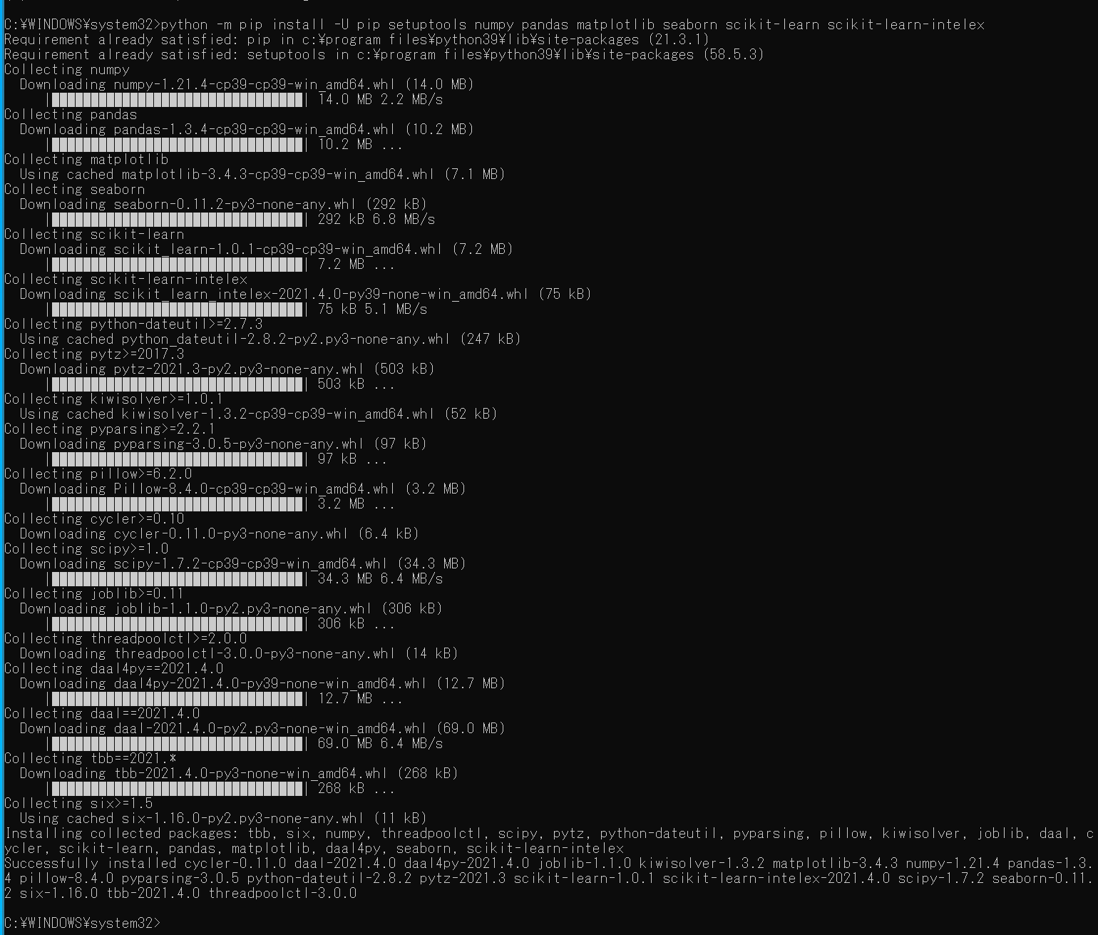
起動したコマンドプロンプトで以下を実行する。
python -m pip install -U --no-user pip setuptools numpy pandas matplotlib seaborn scikit-learn
5. 実行のための準備とその確認手順(Windows 前提)
5.1 プログラムファイルの準備
第7章の演習で示すコードをテキストエディタ(Visual Studio Code やメモ帳など)に貼り付けて保存する(文字コード:UTF-8)。
5.2 実行コマンド
コマンドプロンプトで,保存したプログラムファイルのあるディレクトリに移動し,python に続けてそのファイル名を指定して実行する.
5.3 動作確認チェックリスト
| 確認項目 | 期待される結果 |
|---|---|
| Iris データセットの読み込み | iris.head() により先頭5行が表示される |
| データの形と次元の確認 | iris.shape が (150, 5),iris.ndim が 2 と表示される |
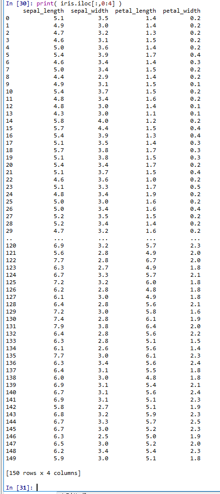
| 0〜3 列目の表示 | iris.iloc[:,0:4] により 150 行 × 4 列の数値データが表示される |
| VBGMM によるクラスタリング | bgmm.predict(X) により 150 個のクラスタラベル(整数)が表示される |
| 各クラスタの重みの確認 | 重みが 0.01 を超えるクラスタのみが番号と重み付きで表示される |
| クラスタリング結果のプロット | PCA による2次元散布図が表示され,クラスタごとに色分けされている |
| Iris データセットのプロット(比較用) | PCA による2次元散布図が表示され,品種(species)ごとに色分けされている |
6. 概要・使い方・実行上の注意
6.1 Iris データセット
Iris データセットは seaborn の load_dataset 関数で読み込む.サイズは 150 × 5,次元数は 2 である.最後の列(species)は花の品種を表す.クラスタリングには 0〜3 列目(sepal_length, sepal_width, petal_length, petal_width)を使用する.
6.2 VBGMM によるクラスタリング
BayesianGaussianMixture に最大クラスタ数(n_components=10)を指定し,fit でモデルを学習させた後,predict で各データ点のクラスタラベルを取得する.random_state=42 を指定し,実行結果の再現性を確保している.
6.3 クラスタの重みの確認
VBGMM は,データに適合するクラスタにだけ大きな重みを割り当てる.bgmm.weights_(各クラスタの重みを並べた配列)を参照し,重みが 0.01 を超えるクラスタを表示することで,有効クラスタ数を確認できる.
6.4 主成分分析による可視化
クラスタリング結果は,PCA で2次元に次元削減し散布図で可視化する.pcaplot 関数は,PCA を適用し第1・第2主成分を軸とする散布図を描画する.ラベルごとに色分けし凡例を表示する.クラスタリング結果と元の品種ラベルのプロットを比較することで,VBGMM の分類のようすを視覚的に確認できる.
7. 演習:VBGMM による Iris データのクラスタリングと可視化
テーマ名:VBGMM を用いた Iris データのクラスタリングと,PCA による結果の可視化.
手順:次のコードを順に実行する(メモ帳を用いる場合は a.py のようなファイル名で保存して実行)。各コードは上から順に同じプログラムとして実行することを想定している.
Iris データセットを読み込み,データの確認を行う.
import numpy as np
import pandas as pd
import matplotlib.pyplot as plt
import seaborn as sns
from sklearn.decomposition import PCA
from sklearn.mixture import BayesianGaussianMixture

sns.set()
iris = sns.load_dataset('iris')
print(iris.head())
形と次元を確認する.サイズは 150 × 5,次元数は 2.最後の列(species)は花の品種を表すデータである.
print(iris.shape)
print(iris.ndim)
Iris データセットの 0, 1, 2, 3 列目を表示する.
print(iris.iloc[:, 0:4])
散布図への主成分分析プロットを準備する.
# 主成分分析で n 個の成分を得る
def prin(A, n):
    return PCA(n_components=n).fit_transform(A)

# M の最初の 2 列を,b で色分けしてプロット.b はラベル
def scatter_label_plot(M, b, alpha):
    a12 = pd.DataFrame(M[:, 0:2], columns=['a1', 'a2'])
    f = pd.factorize(b)
    a12['target'] = f[0]
    g = sns.scatterplot(x='a1', y='a2', hue='target', data=a12, palette=sns.color_palette("hls", np.max(f[0]) + 1), legend="full", alpha=alpha)
    for i, label in enumerate(f[1]):
        g.legend_.get_texts()[i].set_text(label)
    plt.show()

# 主成分分析プロット
def pcaplot(A, b, alpha):
    scatter_label_plot(prin(A, 2), b, alpha)
Iris データセットの 0〜3 列目について,VBGMM でクラスタリングを行う.
X = iris.iloc[:, 0:4].values
bgmm = BayesianGaussianMixture(n_components=10, random_state=42).fit(X)
c = bgmm.predict(X)
print(c)
各クラスタの重みを確認する.
for i, w in enumerate(bgmm.weights_):
    if w > 0.01:
        print(f"クラスタ {i}: 重み {w:.4f}")
結果をプロットする.
pcaplot(X, c, 1)
比較のため,Iris データセットを品種ラベルでプロットする.
pcaplot(X, iris.iloc[:, 4], 1)
ヒント:重みを表示するループでは,0.01 を超える重みを持つクラスタだけが出力される.出力されたクラスタの個数が,VBGMM が実際に使った有効クラスタ数の目安になる.
考察ポイント:有効クラスタ数として表示された個数が,Iris の品種数(3)とどの程度一致するかを確認する.また,クラスタリング結果の散布図と品種ラベルの散布図を見比べ,色分けの対応関係がどの程度合っているかを読み取る.
8. まとめ
8.1 VBGMM によるクラスタ数の自動推定
VBGMM では,クラスタ数を指定せずにクラスタリングを行う.最大クラスタ数を指定しておくと,データに適合するクラスタにだけ大きな重みが割り当てられ,有効なクラスタ数が自動的に決定される.
8.2 クラスタの重みによる有効クラスタの判定
bgmm.weights_ を参照することで各クラスタの重みを確認できる.重みが 0 に近いクラスタは実質的に使用されておらず,これにより有効クラスタ数を把握できる.
8.3 主成分分析(PCA)による可視化
PCA で2次元に次元削減した散布図により,クラスタリング結果を可視化する.元の品種ラベルによるプロットと比較することで,VBGMM の分類のようすを視覚的に確認できる.