画像データの拡張，CIFAR 10 の画像分類を行う畳み込みニューラルネットワークの学習（Keras の前処理層を用いてデータ拡張，MobileNetV2，TensorFlow データセットの CIFAR-10 データセットを使用）（Google Colaboratory へのリンク有り）

【概要】

CIFAR-10 データセット（下図）の画像分類を行う．所定の 10種類に画像分類を行うものである．その 10種類は，airplane, automobile, bird, cat, deer, dog, frog, horse, ship, truck である．

教師データとして用いる画像データの拡張を行う．データ拡張では，Keras の前処理層（RandomFlip，RandomZoom，RandomTranslation）を使い，画像を左右反転する，拡大縮小する，平行移動することを行う．前提として，このページの手順では，データ拡張後の画像データがメモリに入り切る分量であるとしている． TensorFlow データセットのCIFAR-10 データセットを使用する． CNN としては，次のものを使用する．

MobileNetV2 （arxiv: https://arxiv.org/abs/1801.04381）

【目次】

1. Google Colaboratory での実行
2. Windows での実行
3. CIFAR-10 データセットのロード
4. CIFAR-10 データセットの確認
5. CIFAR-10 データセットのデータ拡張
6. ニューラルネットワークの作成（MobileNetV2 を使用）
7. ニューラルネットワークの学習（MobileNetV2 を使用）

【関連する外部ページ】

Keras で利用できる学習済みモデルのページ: https://keras.io/api/applications/
Keras の前処理層のページ: https://keras.io/api/layers/preprocessing_layers/

【サイト内の関連情報】

CNN による画像分類: https://www.kkaneko.jp/ai/imclassify/index.html
tf.image を用いてデータ拡張を行う手順: 別ページ »で説明．データ拡張の部分だけが異なる．
関連の用語集: https://www.kkaneko.jp/tools/man/man.html

1. Google Colaboratory での実行

Google Colaboratory のページ:

次のリンクをクリックすると，Google Colaboratory のノートブックが開く．そして，Google アカウントでログインすると，ノートブック内のコード等を編集したり再実行したりができる．編集した場合でも，他の人に影響が出ることはない．編集後のものを，各自の Google ドライブ内に保存することもできる．

https://colab.research.google.com/drive/1osVlD5wpv-pFMrIt2WgXWbTB8t5fKu9f?usp=sharing

2. Windows での実行

Python 3.12 のインストール

Pythonのインストールを行い、Pythonのプログラムを実行する環境を整える。扱う環境は、Windows搭載パソコンである。金子研究室では、Python 3.12.10を推奨する。

[Windows での Python 3.12 のインストール手順を見るには、ここをクリック]

Windows での Python 3.12 のインストール

以下のいずれかの方法でPython 3.12をインストールする。Pythonがインストール済みの場合、この手順は不要である。

方法 1：winget によるインストール

【インストールコマンドの実行方法】

管理者権限でコマンドプロンプトを起動する（手順：Windowsキーまたはスタートメニュー → cmd と入力 → 右クリック → 「管理者として実行」）。そして、コマンド全体をコマンドプロンプトにコピー＆ペーストする。

--scope machine を指定することで、システム全体（全ユーザー向け）にインストールされる。このオプションの実行には管理者権限が必要である。インストール完了後、コマンドプロンプトを再起動するとPATHが反映される。

REM Python 3.12 をシステム領域にインストール
winget install --id Python.Python.3.12 -e --scope machine --silent --accept-source-agreements --accept-package-agreements --override "/quiet InstallAllUsers=1 PrependPath=1 Include_test=0 Include_pip=1 Include_launcher=1 InstallLauncherAllUsers=1 TargetDir=\"C:\Program Files\Python312\""

REM Python と Scripts を PATH 先頭に追加
powershell -NoProfile -Command "$p='C:\Program Files\Python312'; $s=\"$p\Scripts\"; $c=[Environment]::GetEnvironmentVariable('Path','Machine'); if((Test-Path $p) -and (';'+$c+';' -notlike \"*;$p;*\") -and (';'+$c+';' -notlike \"*;$s;*\")){[Environment]::SetEnvironmentVariable('Path',\"$p;$s;$c\",'Machine')}"

方法 2：インストーラーによるインストール

Python公式サイト（https://www.python.org/downloads/）にアクセスし、「Download Python 3.x.x」ボタンからWindows用インストーラーをダウンロードする。
ダウンロードしたインストーラーを実行する。
初期画面の下部に表示される「Add python.exe to PATH」にチェックを入れてから「Customize installation」を選択する。このチェックを入れ忘れると、コマンドプロンプトから python コマンドを実行できない。
「Install Python 3.xx for all users」にチェックを入れ、「Install」をクリックする。

インストールの確認

コマンドプロンプトで以下を実行する。

python --version

バージョン番号（例：Python 3.12.x）が表示されればインストール成功である。「'python' は、内部コマンドまたは外部コマンドとして認識されていません。」と表示される場合は、インストールが正常に完了していない。

TensorFlow，Keras のインストール

Windows での TensorFlow，Keras のインストール: 別ページ »で説明

（このページで，Build Tools for Visual Studio 2026，NVIDIA ドライバ， NVIDIA CUDA ツールキット， NVIDIA cuDNN のインストールも説明している．）

TensorFlow 2.11 以降は，Windows のネイティブ環境では GPU に対応していない（Windows で GPU を使う場合は WSL2 上で動かす）． Windows のネイティブ環境では CPU で動作する．出典: https://www.tensorflow.org/install/pip

Graphviz のインストール

Windows での Graphviz のインストール: 別ページ »で説明

numpy，matplotlib，seaborn，scikit-learn，pandas，pydot のインストール

管理者権限でコマンドプロンプトを起動する（手順：Windowsキーまたはスタートメニュー → cmd と入力 → 右クリック → 「管理者として実行」）。

次のコマンドを実行する．

python -m pip install -U --no-user numpy matplotlib seaborn scikit-learn pandas pydot

3. CIFAR-10 データセットのロード

パッケージのインポート，TensorFlow のバージョン確認など

import tensorflow as tf
import numpy as np
import tensorflow_datasets as tfds
tf.keras.backend.clear_session()

%matplotlib inline
import matplotlib.pyplot as plt
import warnings
warnings.filterwarnings('ignore')   # Matplotlib の警告メッセージを表示しない

# TensorFlow のバージョンを表示
print(tf.__version__)

# GPU が使えるときは，GPU のメモリを必要に応じて確保する設定にする
gpus = tf.config.list_physical_devices(device_type='GPU')
if len(gpus) > 0:
    print(f">> GPU detected. {gpus[0].name}")
    tf.config.experimental.set_memory_growth(gpus[0], True)

CIFAR-10 データセットのロード
tensorflow_datasets の load で，「batch_size = -1」を指定して，一括読み込みを行っている．
```
cifar10, cifar10_info = tfds.load('cifar10', with_info=True, shuffle_files=True, as_supervised=True, batch_size=-1)
```

4. CIFAR-10 データセットの確認

データセットの中の画像を表示

Matplotlib を用いて，0 番目の画像を表示する

%matplotlib inline
import matplotlib.pyplot as plt
import warnings
warnings.filterwarnings('ignore')   # Matplotlib の警告メッセージを表示しない
NUM = 0
# NUM 番目の画像を表示
plt.imshow(cifar10['train'][0][NUM])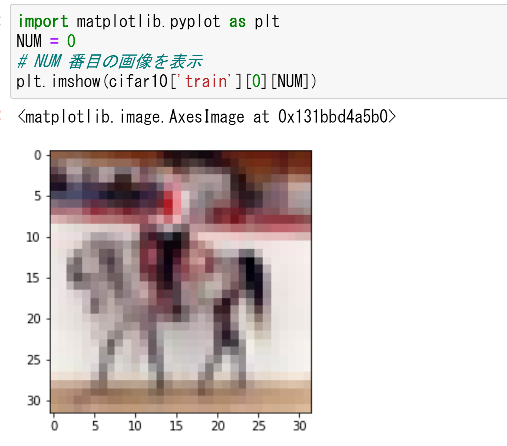

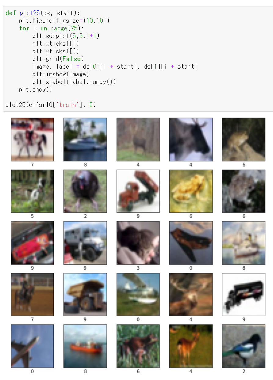
Matplotlib を用いて，複数の画像を並べて表示する．

def plot25(ds, start):
    plt.figure(figsize=(10, 10))
    for i in range(25):
        plt.subplot(5, 5, i + 1)
        plt.xticks([])
        plt.yticks([])
        plt.grid(False)
        image, label = ds[0][i + start], ds[1][i + start]
        plt.imshow(image)
        plt.xlabel(label.numpy())
    plt.show()

plot25(cifar10['train'], 0)

データセットの情報を表示

print(cifar10_info)
print(cifar10_info.features["label"].num_classes)
print(cifar10_info.features["label"].names)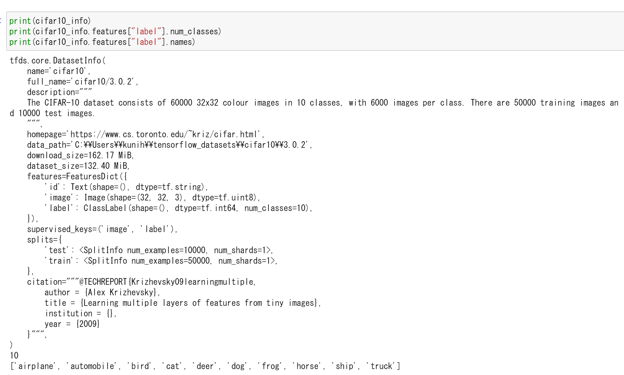

cifar10['train'] と cifar10['test'] の形と次元を確認
cifar10['train']: サイズ 32 かける 32 の 50000枚のカラー画像，50000枚のカラー画像それぞれのラベル（0 から 9 のどれか）
cifar10['test']: サイズ 32 かける 32 の 10000枚のカラー画像，10000枚のカラー画像それぞれのラベル（0 から 9 のどれか）
```
print(cifar10['train'][0].shape)
print(cifar10['train'][1].shape)
print(cifar10['test'][0].shape)
print(cifar10['test'][1].shape)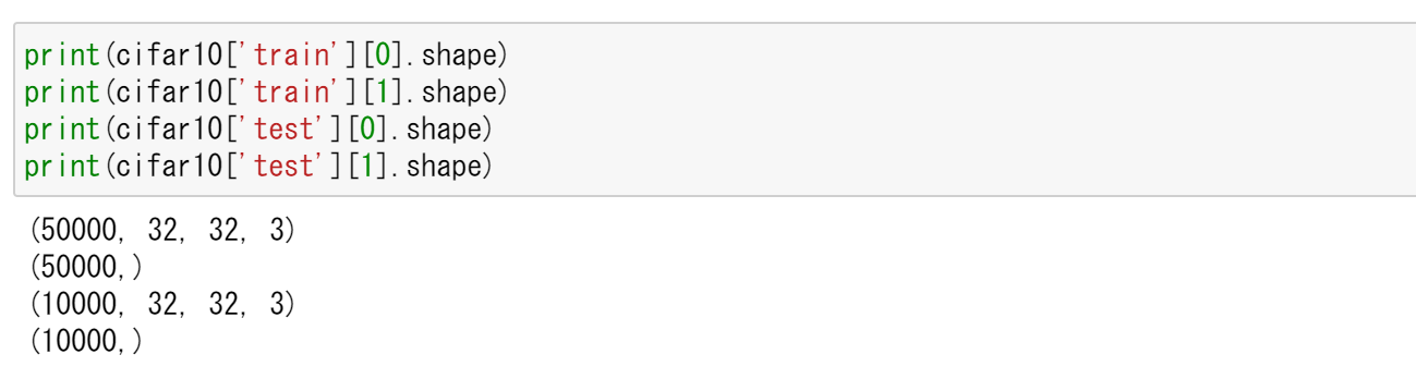
```

5. CIFAR-10 データセットのデータ拡張

データセットの生成

ds_train, ds_test = cifar10['train'], cifar10['test']

ニューラルネットワークを使うために，データの前処理
値は，もともと int で 0 から 255 の範囲であるのを， float32 で 0 から 1 の範囲になるように前処理を行う．
```
ds_train = (ds_train[0].numpy().astype("float32") / 255., ds_train[1])
ds_test = (ds_test[0].numpy().astype("float32") / 255., ds_test[1])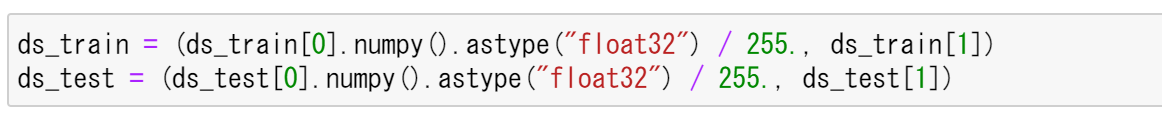
```

画像データの拡張を行ってみる

画像データは，ds_train[0] にある． Keras の前処理層を使い，画像を左右反転する，拡大縮小する，平行移動することを行う． ds_train[1] にはラベルのデータが入っているとする．

結果の入る augmented_ds_train はタプル（複数の値を組にしたもの）．うち 1つ目は numpy の配列，2つ目は要素が tf.Tensor の配列．

# データ拡張を行う関数オブジェクトを生成
def gen_data_augmentation(seed):
    data_augmentation = tf.keras.Sequential(
        [
            tf.keras.layers.RandomFlip("horizontal", seed=seed),
            tf.keras.layers.RandomZoom(height_factor=(-0.1, 0.1), width_factor=(-0.1, 0.1), seed=seed),
            tf.keras.layers.RandomTranslation(height_factor=(-0.1, 0.1), width_factor=(-0.1, 0.1), fill_mode='wrap', seed=seed)
        ]
    )
    return data_augmentation

# 複数画像を一括してデータ拡張
def augment_images(images, seed):
    data_augmentation = gen_data_augmentation(seed)
    a = [*map(lambda x: np.squeeze(data_augmentation(x[np.newaxis, ...], training=True), 0), images)]
    return np.array(a)

augmented_ds_train = (augment_images(ds_train[0], seed=0), ds_train[1])
plot25(augmented_ds_train, 0)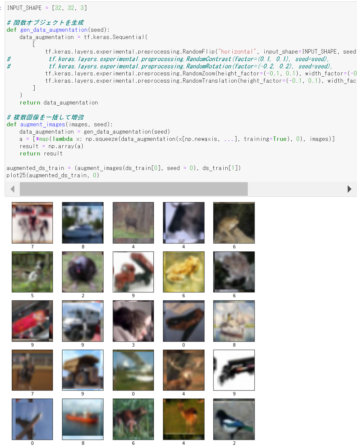

画像データが増えたことの確認
```
print(augmented_ds_train[0].shape)
```

今度は，画像データの拡張を行いながら，画像データを 5倍に増やす．

ここで増やした画像データは，あとで使用する．

def increase_image_data(ds_train, t):
# t 倍に増やす
    x1 = augment_images(ds_train[0], 1)
    y1 = ds_train[1]
    if t > 1:
        for i in range(t - 1):
            x2 = augment_images(ds_train[0], i + 2)
            # 画像は nparray, ラベルは tf.Tensor を要素とする配列にする
            x1 = np.concatenate([x1, x2])
            y1 = tf.concat([y1, ds_train[1]], axis=0)

    return (x1, y1)

augmented_ds_train = increase_image_data(ds_train, 5)
plot25(augmented_ds_train, 0)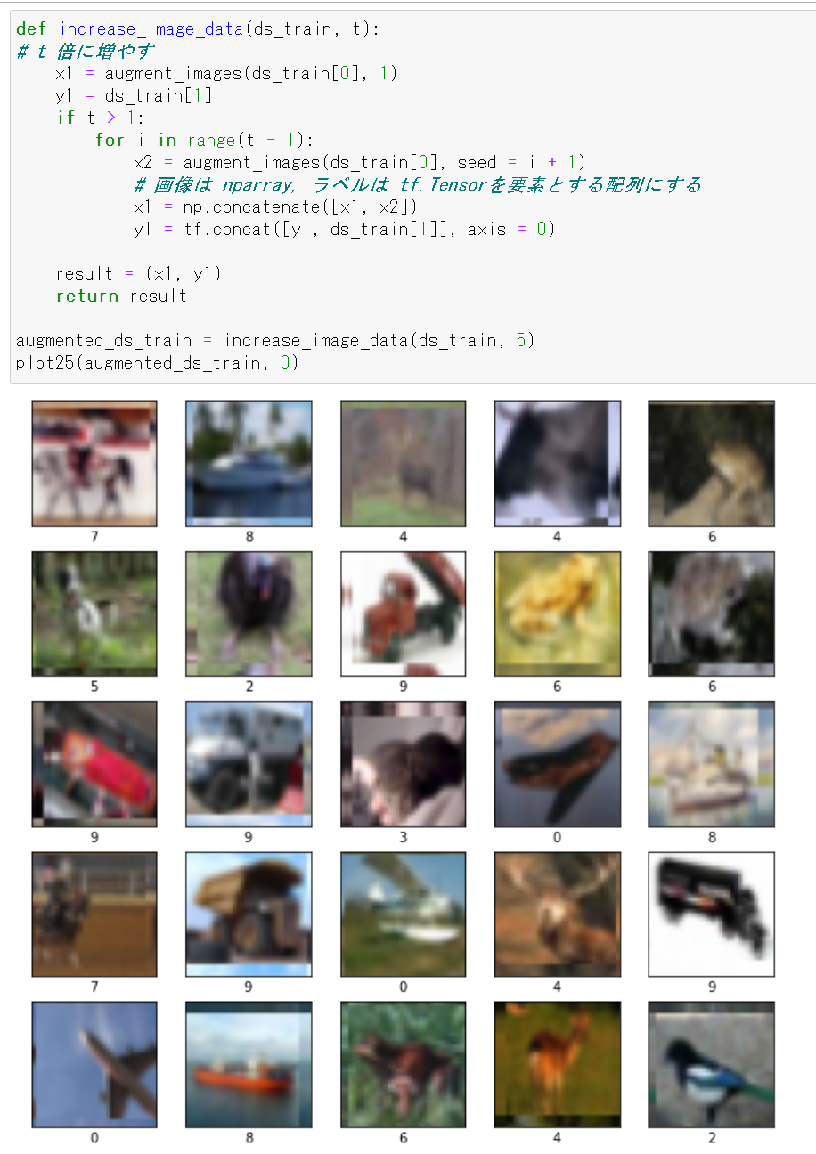

6. ニューラルネットワークの作成（MobileNetV2 を使用）

ニューラルネットワークの作成と確認とコンパイル
Keras の MobileNetV2 を使う．「weights=None」を指定することにより，最初，重みはランダムに設定する．

オプティマイザと損失関数とメトリクスを設定する．
- Keras のオプティマイザのページ: https://keras.io/api/optimizers/
- Keras の損失関数のページ: https://keras.io/api/losses/
- Keras のメトリクスのページ: https://keras.io/api/metrics/
```
NUM_CLASSES = 10
INPUT_SHAPE = (32, 32, 3)
m1 = tf.keras.applications.mobilenet_v2.MobileNetV2(input_shape=INPUT_SHAPE, weights=None, classes=NUM_CLASSES)
m1.summary()
m1.compile(
    optimizer=tf.keras.optimizers.Adam(learning_rate=0.001),
    loss='sparse_categorical_crossentropy',
    metrics=['sparse_categorical_crossentropy', 'accuracy'])
```
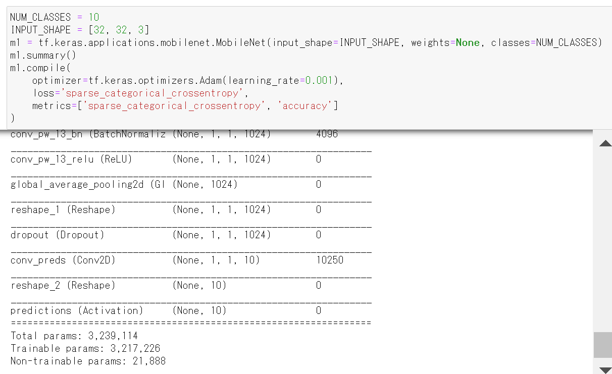
モデルのビジュアライズ
Keras のモデルのビジュアライズについては: https://keras.io/api/utils/model_plotting_utils/
ここでの表示でエラーメッセージが出る場合でも，モデル自体は問題なくできていると考えられる．続行する．
```
from tensorflow.keras.utils import plot_model
plot_model(m1)
```

7. ニューラルネットワークの学習（MobileNetV2 を使用）

使用するデータの確認

print(augmented_ds_train[0].shape)
print(augmented_ds_train[1].shape)
print(ds_test[0].shape)
print(ds_test[1].shape)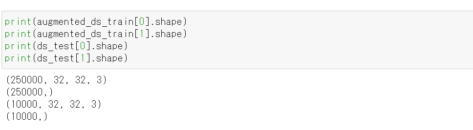

ニューラルネットワークの学習を行う

ニューラルネットワークの学習は fit メソッドにより行う．教師データを投入する．

epochs = 20
history = m1.fit(augmented_ds_train[0], augmented_ds_train[1],
                 epochs=epochs,
                 validation_data=(ds_test[0], ds_test[1]),
                 verbose=1)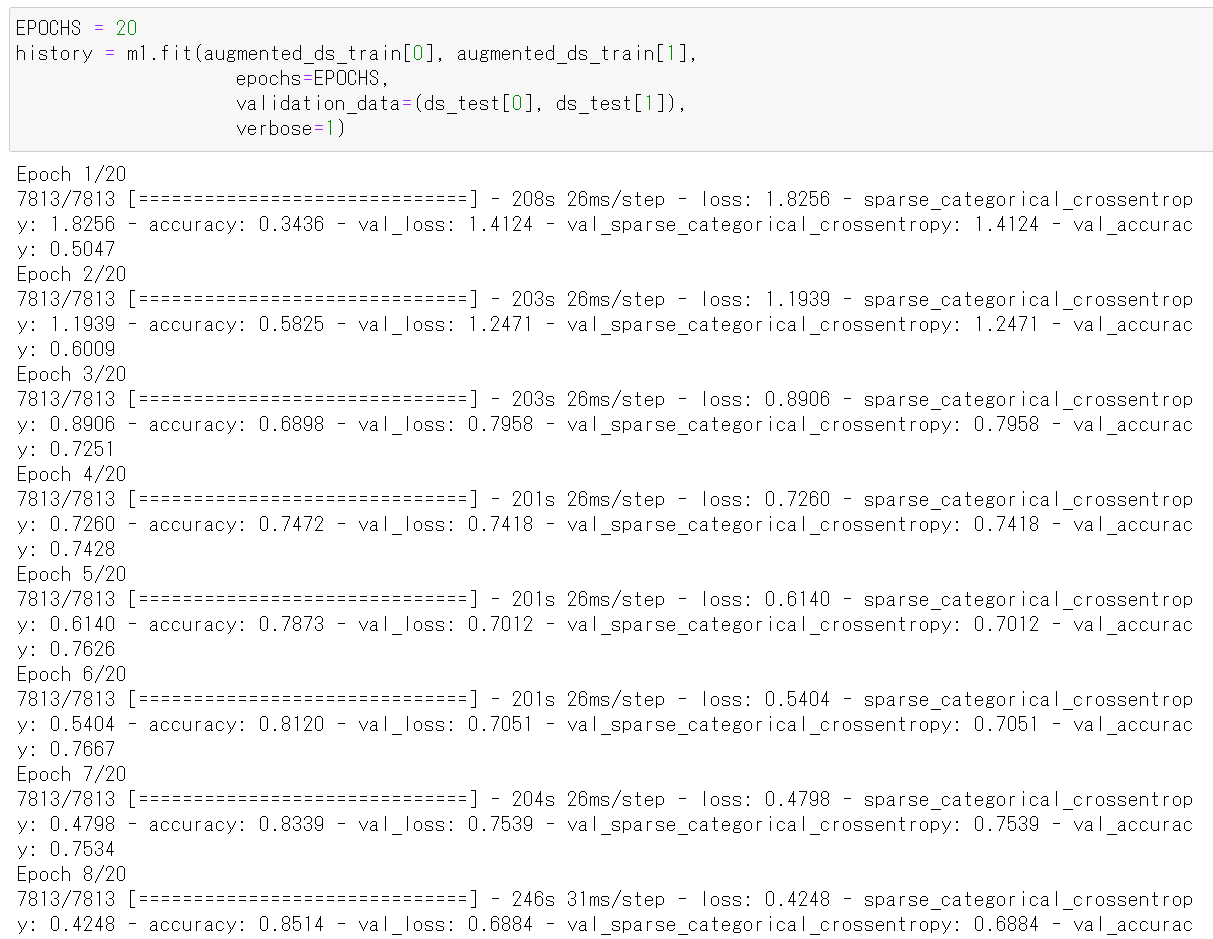

CNN による画像分類
ds_test を分類してみる．
```
print(m1.predict(ds_test[0]))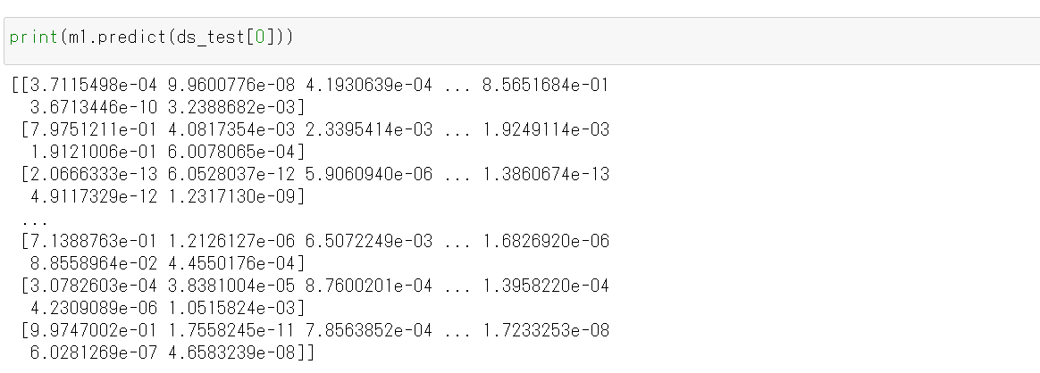
```
それぞれの数値の中で，一番大きいものはどれか．
```
m1.predict(ds_test[0]).argmax(axis=1)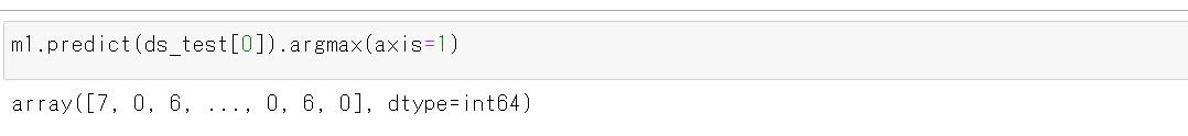
```
ds_test 内にある正解のラベル（クラス名）を表示する（上の結果と比べるため）．
```
print(ds_test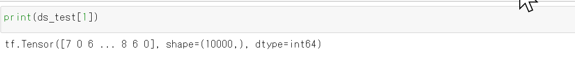[1])
```

学習曲線の確認

過学習や学習不足について確認．

import pandas as pd
hist = pd.DataFrame(history.history)
hist['epoch'] = history.epoch
print(hist)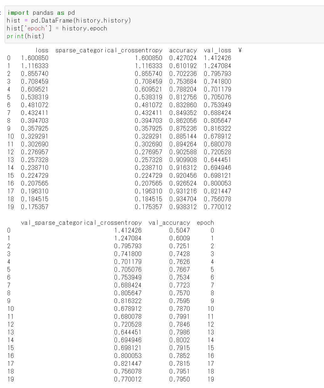

学習曲線のプロット

過学習や学習不足について確認．

https://www.tensorflow.org/tutorials/keras/overfit_and_underfit?hl=ja で公開されているプログラムを使用

%matplotlib inline
import matplotlib.pyplot as plt
import warnings
warnings.filterwarnings('ignore')   # Matplotlib の警告メッセージを表示しない
def plot_history(histories, key='binary_crossentropy'):
  plt.figure(figsize=(16,10))

  for name, history in histories:
    val = plt.plot(history.epoch, history.history['val_'+key],
                   '--', label=name.title()+' Val')
    plt.plot(history.epoch, history.history[key], color=val[0].get_color(),
             label=name.title()+' Train')

  plt.xlabel('Epochs')
  plt.ylabel(key.replace('_',' ').title())
  plt.legend()

  plt.xlim([0,max(history.epoch)])


plot_history([('history', history)], key='sparse_categorical_crossentropy')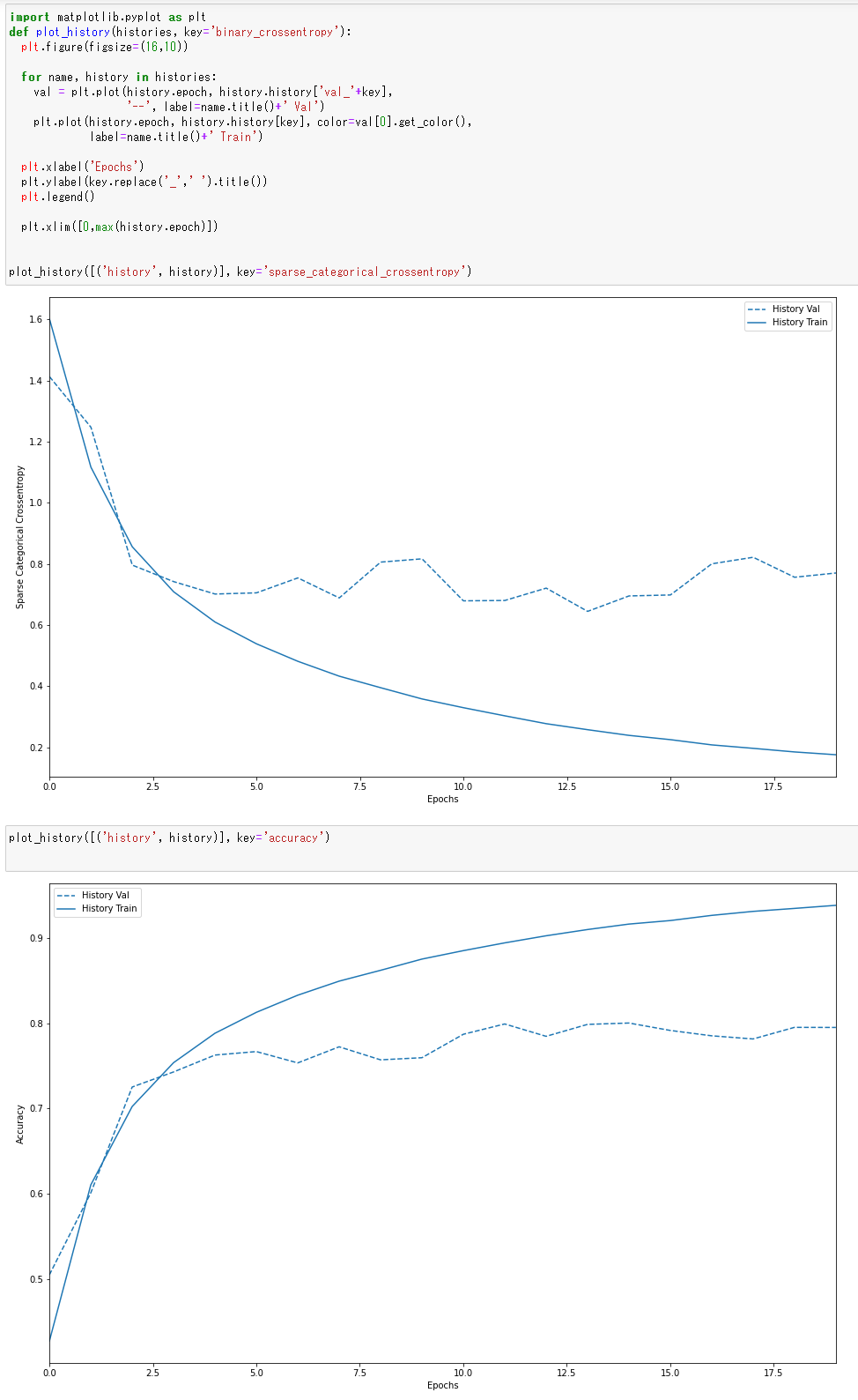

plot_history([('history', history)], key='accuracy')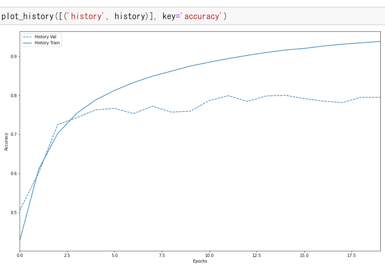

データ拡張を行わない場合の結果（学習曲線など）は，別ページ »で説明