人工知能,データサイエンス,統計,コンピュータビジョンの用語集
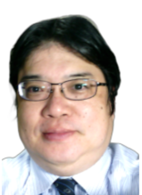
300W (300 Faces-In-The_Wild) データセット
顔のデータベース、顔の 68 ランドマークが付いている。
【文献】
C. Sagonas, G. Tzimiropoulos, S. Zafeiriou and M. Pantic, "300 Faces in-the-Wild Challenge: The First Facial Landmark Localization Challenge," 2013 IEEE International Conference on Computer Vision Workshops, 2013, pp. 397-403, doi: 10.1109/ICCVW.2013.59.
https://ibug.doc.ic.ac.uk/media/uploads/documents/sagonas_2016_imavis.pdf
【関連する外部ページ】
- 300 Faces In-The-Wild Challenge のページ: https://ibug.doc.ic.ac.uk/resources/300-W/
- OpenMMLab の 300W データセット: https://github.com/open-mmlab/mmpose/blob/master/docs/en/tasks/2d_face_keypoint.md#300w-dataset
【関連項目】 HELEN データセット, iBUG 300-W データセット, face alignment, 顔ランドマーク (facial landmark)の検出, 3次元の顔の再構成 (3D face reconstruction), OpenMMLab, 顔の 68 ランドマーク, 顔のデータベース
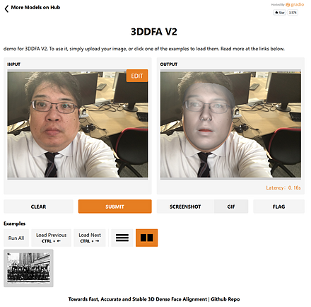
3DDFA_V2
3DDFA_V2 は、 3次元の顔の再構成 (3D face reconstruction) のうち dense vertices regression を行う一手法。論文は、2020年発表。
【文献】
Jianzhu Guo, Xiangyu Zhu, Yang Yang, Fan Yang, Zhen Lei, Stan Z. Li, Towards Fast, Accurate and Stable 3D Dense Face Alignment, ECCV 2020.
https://arxiv.org/pdf/2009.09960v2.pdf
【関連する外部ページ】
- GitHub のページ: https://github.com/cleardusk/3DDFA_V2
-
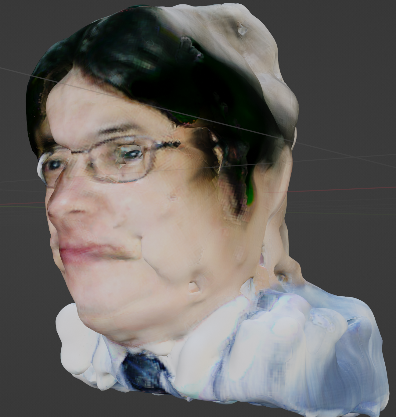
Hugging Face での 3DDFA_V2 のオンライン実行
URL: https://huggingface.co/spaces/PKUWilliamYang/3DDFA_V2
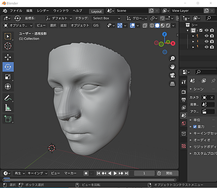
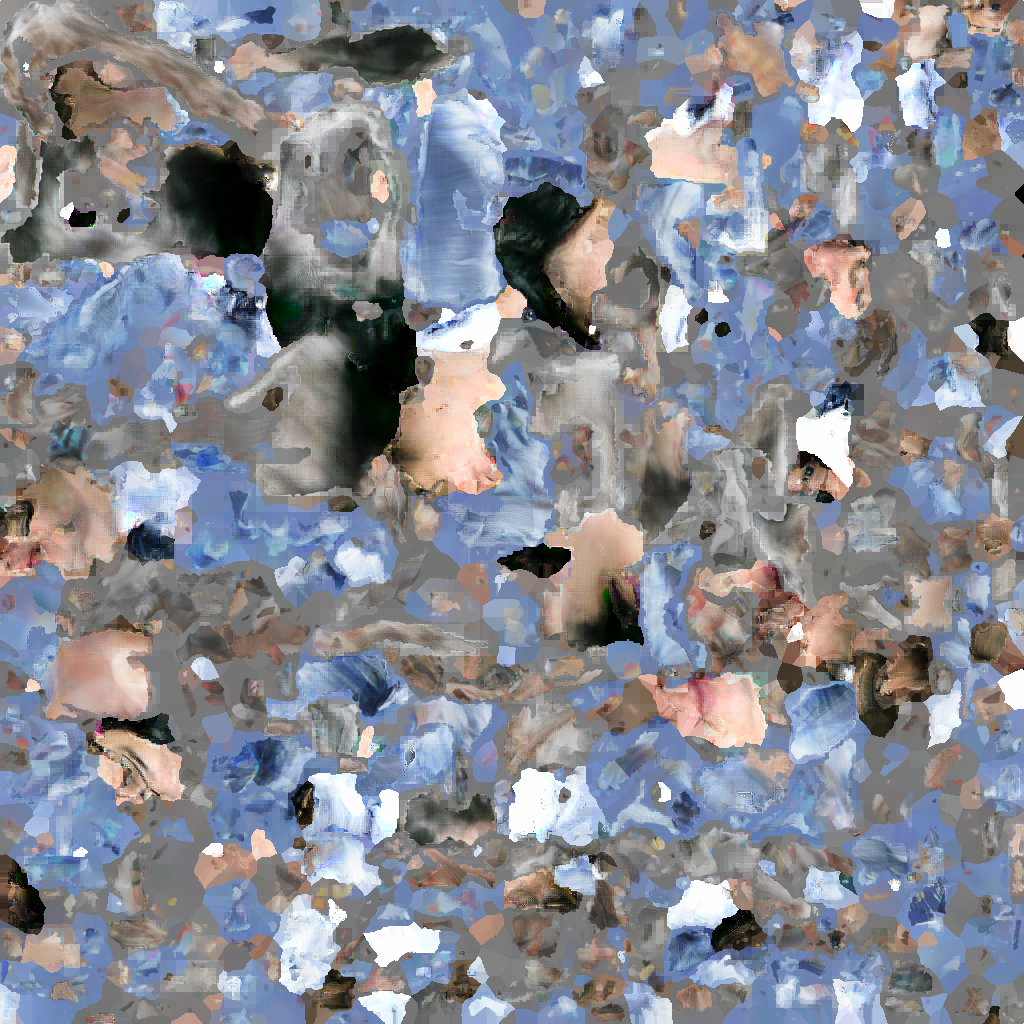
作成された3次元モデルを Blender にインポートした画面。
Google Colaboratory での 3DDFA_V2 のオンライン実行
次のページでは、Google Colaboratory で実行できるプログラムコード、プログラム利用ガイド、プログラムコードの説明など示している。
URL: https://www.kkaneko.jp/ai/intro/3ddfav2.html
【概要】本記事では、3DDFA_V2フレームワークを用いた3次元顔モデル生成プログラムについて解説する。単一の顔画像から3次元形状を復元し、OBJ/PLY形式で出力する技術をGoogle Colab環境で提供する。
Colabのページ(ソースコードと説明): https://colab.research.google.com/drive/1fNfAdCRxnxxcxj9mH7lFVsP-uz4DAWoV?usp=sharing
3次元姿勢推定 (3D pose estimation)
画像から、物体検出を行うとともに、その3次元の向きの推定も行う。
【関連項目】 Objectron
3次元の顔の再構成 (3D face reconstruction)
3次元の顔の再構成 (3D face reconstruction) は、 顔の写った画像から、元の顔の3次元の形を構成すること。
3次元の顔の再構成は、次の2つの種類がある。
- 3次元の変形可能な顔のモデル (3D Morphable Model) について、そのパラメータを、画像を使って推定すること。 FaceRig などが有名である。
- dense vertices regression: dense は「密な」、vertices は「頂点」、regression は「回帰」。画像から、顔の3次元データであるポリゴンメッシュを推定する
3次元再構成 (3D reconstruction)
3次元再構成 (3D reconstruction) の機能をもつソフトウェアとしては、 colmap、 Meshroom がある。
【関連項目】 colmap, Meshroom, Multi View Stereo, OpenMVG, OpenMVS, Structure from Motion
AdaDelta 法
M.Zeiler の AdaDelta 法は、学習率をダイナミックに変化させる技術。 学習率をダイナミックに変化させる技術は、その他 Adam 法なども知られる。
確率的勾配降下法 (SGD 法) をベースとしているが、 確率的勾配降下法が良いのか、Adadelta 法が良いのかは、一概には言えない。
from tensorflow.keras.optimizers import Adadelta
optimizer = Adadelta(rho=0.95)
M. Zeiler, Adadelta An adaptive learning rate method, 2012.
Adam 法
Adam 法は、学習率をダイナミックに変化させる技術。 学習率をダイナミックに変化させる技術は、その他 AdaDelta 法なども知られる。 Adam 法を使うプログラム例は次の通り。
m.compile(
    optimizer=tf.keras.optimizers.Adam(learning_rate=0.001),
    loss='sparse_categorical_crossentropy',
    metrics=['sparse_categorical_crossentropy', 'accuracy']
)
Diederik Kingma and Jimmy Ba, Adam: A Method for Stochastic Optimization, 2014, CoRR, abs/1412.6980
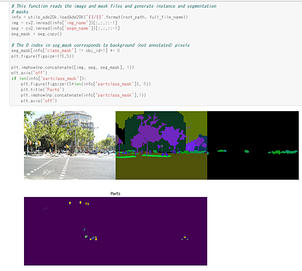
ADE20K データセット
ADE20K データセット は、 セマンティック・セグメンテーション、シーン解析(scene parsing)、 インスタンス・セグメンテーション (instance segmentation)についてのアノテーション済みの画像データセットである。
次の特色がある
- データの多様性
- 画素単位でのアノテーション
- オブジェクト(car や person など) も、背景領域も(grass, sky など) アノテーションされている。
- 腕や足などの、オブジェクトのパーツ (object parts) もアノテーションされている。
画像数、オブジェクト数などは次の通り。
- 画像数: 30,574 枚
うち学習用: 25,574 枚、 うち検証用: 2,000 枚、 うちテスト用: 3,000 枚。
- オブジェクト数: 707,868
- オブジェクトのカテゴリ数: 3,688
- アノテーションされたオブジェクトのパーツ (object parts) : 193,238
利用には、次の URL で登録が必要。
ADE20K データセットの URL: http://groups.csail.mit.edu/vision/datasets/ADE20K/
【文献】
- Bolei Zhou, Hang Zhao, Xavier Puig, Sanja Fidler, Adela Barriuso, Antonio Torralba, Scene Parsing Through ADE20K Dataset, CVPR 2017, also CoRR, abs/1608.05442, 2017.
- Bolei Zhou, Hang Zhao, Xavier Puig, Tete Xiao, Sanja Fidler, Adela Barrieso and Antonio Torralba, Semantic Understanding of Scenes through ADE20K Dataset, International Journal on Computer Vision (IJCV), also CoRR, abs/1608.05442v2, 2016.
【関連する外部ページ】
- ADE20K データセットの URL: http://groups.csail.mit.edu/vision/datasets/ADE20K/
- CSAILVision の ADE20K のページ (GitHub のページ): https://github.com/CSAILVision/ADE20K
- CSAILVision の ADE20K スターターコード のページ (GitHub のページ):
https://github.com/CSAILVision/ADE20K/blob/main/notebooks/ade20k_starter.ipynb
このスターターコードは、画像1枚について元画像とアノテーションを表示するもの
- Papers With Code の ADE20K データセットのページ: https://paperswithcode.com/dataset/ade20k
【関連項目】 セマンティック・セグメンテーション (semantic segmentation), シーン解析(scene parsing), インスタンス・セグメンテーション (instance segmentation), Detectron2, CSAILVision, MIT Scene Parsing Benchmark, 物体検出
AFLW (Annotated Facial Landmarks in the Wild) データセット
AFLW (Annotated Facial Landmarks in the Wild) データセットは、 Flickr から収集された24,386枚の顔画像である。 さまざまな表情、民族、年齢、性別、撮影条件、環境条件の顔が収集されている。 それぞれの顔には、最大21個の顔ランドマークが付けられている。
- 24,386枚の画像。うち、59%が女性、41%が男性である。複数の顔を含む画像もある。 ほとんどの画像がカラーだが、中には、濃淡画像もある。
- 約380,000 の顔について、顔ごとに 21 個の顔ランドマークが付いている。
- 顔で、左耳たぶが見えてないような場合、左耳たぶの顔ランドマークはアノテーションされていない(見えない場合はアノテーションされない)
次の URL で公開されているデータセット(オープンデータ)である。
URL: https://www.tugraz.at/institute/icg/research/team-bischof/lrs-group/downloads
【文献】
M. Köstinger, P. Wohlhart, P. M. Roth and H. Bischof, "Annotated Facial Landmarks in the Wild: A large-scale, real-world database for facial landmark localization," 2011 IEEE International Conference on Computer Vision Workshops (ICCV Workshops), 2011, pp. 2144-2151, doi: 10.1109/ICCVW.2011.6130513.
【関連する外部ページ】
- Papers With Code の AFLW データセットのページ: https://paperswithcode.com/dataset/aflw
- open-mmlab での記事
https://github.com/open-mmlab/mmpose/blob/master/docs/en/tasks/2d_face_keypoint.md#aflw-dataset
AgeDB データセット
手作業で収集された、「in-the-wild」の顔と年齢のデータベース。 年号まで正確に記録された顔画像が含まれている。
次の URL で公開されているデータセット(オープンデータ)である。
https://ibug.doc.ic.ac.uk/resources/agedb/
【文献】
S. Moschoglou, A. Papaioannou, C. Sagonas, J. Deng, I. Kotsia and S. Zafeiriou, "AgeDB: The First Manually Collected, In-the-Wild Age Database," 2017 IEEE Conference on Computer Vision and Pattern Recognition Workshops (CVPRW), 2017, pp. 1997-2005, doi: 10.1109/CVPRW.2017.250.
https://ibug.doc.ic.ac.uk/media/uploads/documents/agedb.pdf
【関連する外部ページ】
【関連項目】 顔認識 (face recognition), 顔のデータベース
AIM-500 (Automatic Image Matting-500) データセット
イメージ・マッティング (image matting) のデータセット。 3種類の前景(Salient Opaque, Salient Transparent/Meticulous, Non-Salient)を含む 500枚の画像について、元画像と alpha matte と Trimap のデータセットである。
次の URL で公開されているデータセット(オープンデータ)である。
URL: https://drive.google.com/drive/folders/1IyPiYJUp-KtOoa-Hsm922VU3aCcidjjz
【文献】
Jizhizi Li, Jing Zhang, DaCheng Tao, Deep Automatic Natural Image Matting, CoRR, abs/2107.07235v1, 2021.
https://arxiv.org/pdf/2107.07235v1.pdf
【関連する外部ページ】
- 公式ページ の URL: https://github.com/JizhiziLi/AIM
- Papers with Code のページ: https://paperswithcode.com/dataset/aim-500
【関連項目】 イメージ・マッティング (image matting), オープンデータ (open data)
AlexeyAB darknet
AlexeyAB darknet は、YOLOv2, YOLOv3, YOLOv4 の機能などを持つ。
【文献】
Chien-Yao Wang, Alexey Bochkovskiy, Hong-Yuan Mark Liao, Scaled-YOLOv4: Scaling Cross Stage Partial Network, Proceedings of the IEEE/CVF Conference on Computer Vision and Pattern Recognition (CVPR) 2021, pp. 13029-13038, also CoRR, Scaled-YOLOv4: Scaling Cross Stage Partial Network, 2021.
https://arxiv.org/pdf/2011.08036v2.pdf
【サイト内の関連ページ】 AlexeyAB/darknet のインストールと動作確認(Scaled YOLO v4 による物体検出)(Windows 上)
【関連する外部ページ】
- Alexey による darknet の実装(GitHub)ページ: https://github.com/AlexeyAB/darknet
- COCO データセットで事前学習済みモデルの重みのデータの URL: https://github.com/AlexeyAB/darknet
【関連項目】 YOLOv3, YOLOv4, RetinaNet, 物体検出
Alexnet
AlexNet の場合
input 3@224x224
conv 11x11
  96@55x55
pooling
conv 5x5
  256@27x27
pooling
  16@5x5
conv 3x3
  384@13x13
conv 3x3
  384@13xx13
conv 3x3
  256@13x13
affine
  4096
affine
  4096
  1000
参考文献: ch08/deep_convnet.py
AltCLIP
AltCLIP の特徴は、 CLIP のテキストエンコーダ (text encoder) を 学習済みの多言語のテキストエンコーダ XLM-R で置き換えたこと。
【文献】
Zhongzhi Chen, Guang Liu, Bo-Wen Zhang, Fulong Ye, Qinghong Yang, Ledell Wu, AltCLIP: Altering the Language Encoder in CLIP for Extended Language Capabilities, arXiv:2211.06679, 2022.
【関連項目】 CLIP
AP
機械学習による物体検出では、 「AP」は、「average precision」の意味である。
Applications of Deep Neural Networks
「Applications of Deep Neural Networks」は、ディープラーニングに関するテキスト。 ニューラルネットワーク、 CNN (convolutional neural network), LSTM (Long Short-Term Memory), GRU (Gated Recurrent Neural Networks), GAN (Generative Adversarial Network), 強化学習とその応用について学ぶことができる。 Python, TensorFlow, Keras を使用している。
【関連する外部ページ】
- Papers with Code のページ: https://paperswithcode.com/paper/applications-of-deep-neural-networks
- PDF ファイル: https://arxiv.org/pdf/2009.05673v3.pdf
【関連項目】 CNN (convolutional neural network), GAN (Generative Adversarial Network), GRU (Gated Recurrent Neural Networks), Keras, LSTM (Long Short-Term Memory), TensorFlow, ディープラーニング ニューラルネットワーク、 強化学習
ArcFace 法
距離学習の1手法である。 分類モデルが特徴ベクトルを生成するための複数の層と、最終層の softmax から構成されているとき、 その分類モデルでの、特徴ベクトルを生成するための複数の層の出力に対して、 L2 正規化の処理と、Angular Magin Penalty 層による処理を追加し、softmax 層につなげる。
deepface, InsightFace などで実装されている。
【文献】
Jiankang Deng, Jia Guo, Niannan Xue, Stefanos Zafeiriou, ArcFace: Additive Angular Margin Loss for Deep Face Recognition, CVPR 2019, also CoRR, abs/1801.07698v3, 2019.
https://arxiv.org/pdf/1801.07698v3.pdf
【関連する外部ページ】
- Papers with Code のページ: https://paperswithcode.com/method/arcface
【関連項目】 deepface, InsightFace, 顔検証 (face verification), 顔識別 (face identification), 顔認識 (face recognition), 顔に関する処理
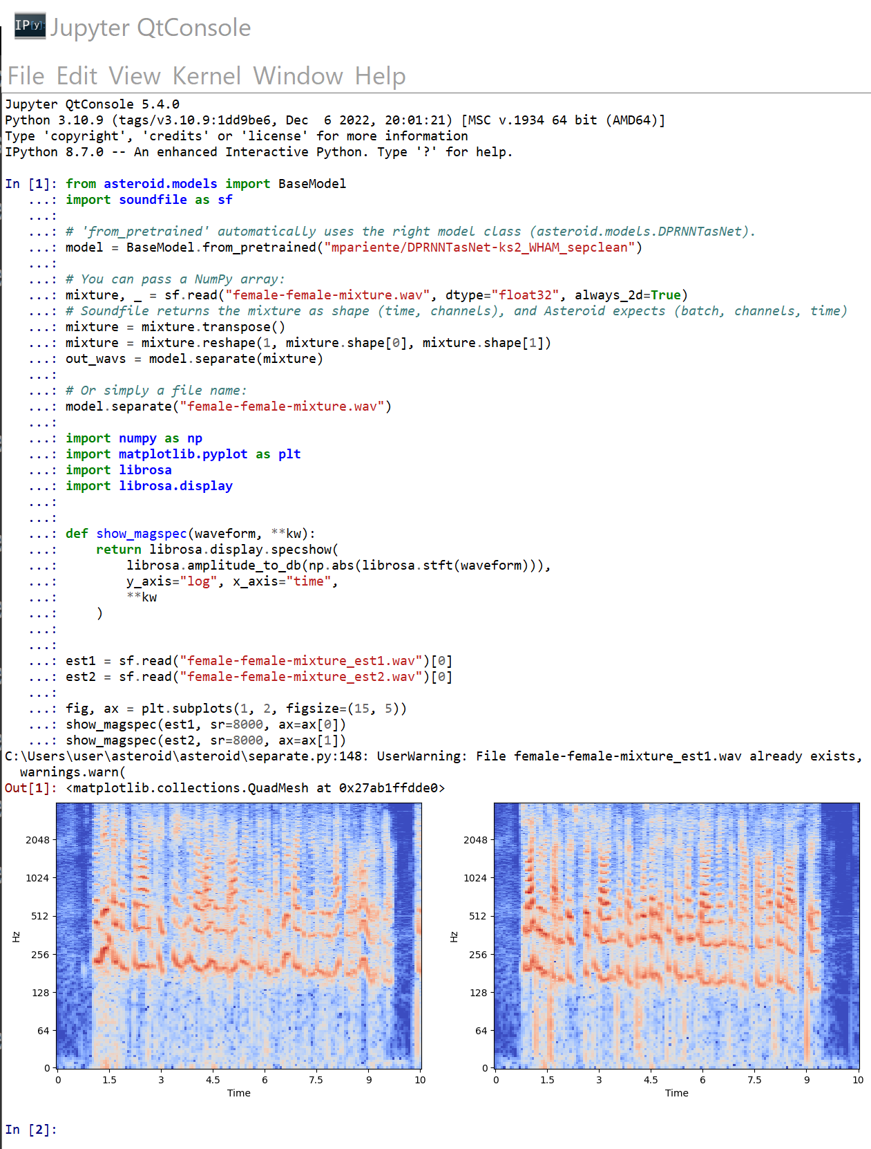
asteroid
asteroid は、音源分離(audio source separation)のツールキット。
【文献】
Ryosuke Sawata, Stefan Uhlich, Shusuke Takahashi, Yuki Mitsufuji, All for One and One for All: Improving Music Separation by Bridging Networks, CoRR, abs/2010.04228v4, 2021.
PDF: https://arxiv.org/pdf/2010.04228v4.pdf
【関連する外部ページ】
- GitHub のページ: https://github.com/asteroid-team/asteroid
- Papers with Code のページ: https://paperswithcode.com/paper/all-for-one-and-one-for-all-improving-music
【関連項目】 audio source separation, music source separation, speech enhancement
Windows での asteroid のインストールと動作確認(音源分離)
asteroid のインストールと動作確認(音源分離)(Python、PyTorch を使用)(Windows 上): 別ページ »で説明
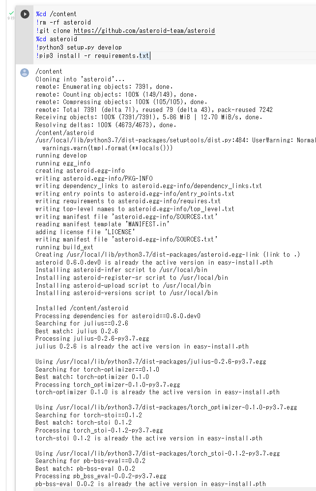
Google Colaboratory での asteroid のインストール
公式の手順 https://github.com/asteroid-team/asteroid による。
次のコマンドやプログラムは Google Colaboratory で動く(コードセルを作り、実行する)。
%cd /content
!rm -rf asteroid
!git clone https://github.com/asteroid-team/asteroid
%cd asteroid
!python3 setup.py develop
!pip3 install -r requirements.txt
AVA
Spatio-Temporal Action Recognition の一手法。2016年発表
- 文献
Gu, Chunhui and Sun, Chen and Ross, David A and Vondrick, Carl and Pantofaru, Caroline and Li, Yeqing and Vijayanarasimhan, Sudheendra and Toderici, George and Ricco, Susanna and Sukthankar, Rahul and others, Ava: A video dataset of spatio-temporally localized atomic visual actions, Proceedings of the IEEE Conference on Computer Vision and Pattern Recognition, pp. 6047--6056, 2018.
- MMAction2 の AVA の説明ページ: https://github.com/open-mmlab/mmaction2/blob/master/configs/detection/ava/README.md
【関連項目】 MMAction2, Spatio-Temporal Action Recognition, 動作認識 (action recognition)
Bark
Bark は Transformer ベースの音声合成の技術。多言語に対応。
【サイト内の関連ページ】
- 多言語の音声合成(Bark、Python、PyTorch を使用)(Windows 上): 別ページ »で説明
【関連する外部ページ】
- Bark の公式の GitHub のページ : https://github.com/suno-ai/bark
- Bark の Paper with Code のページ: https://paperswithcode.com/paper/neural-codec-language-models-are-zero-shot
【関連項目】 VALL-E X
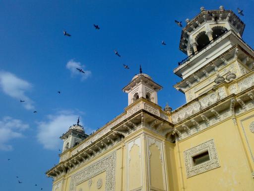
BASNet (Boundary-Aware Salient object detection)
BASNet は、 ディープラーニングにより、Salient Object Detection (顕著オブジェクトの検出)を行う一手法。2019年発表。
BASNet は次の2つのモジュールから構成される。
- Predict Module:
入力画像から saliency map を生成する。 U-Net に類似の構造を持つ、教師有りの Encoder-Decoder ネットワークである。 この段階での saliency map は、粗い (coarse) ものである。
- Residual Refinement Module:
Predict Module が生成した saliency map をリファイン (refine) する。 Residual Refinement Module は Predict Module が生成した saliency map と、正解 (ground truth) との残差 (residuals) を学習する。
Salient Object Detection は、 視覚特性の異なるオブジェクトを、画素単位で切り出す。 前景と背景の分離に役立つ場合がある。人間がマスクの指定や塗り分け(Trimap など)を行うことなく実行される。
【文献】
Qin, Xuebin and Zhang, Zichen and Huang, Chenyang and Gao, Chao and Dehghan, Masood and Jagersand, Martin, BASNet: Boundary-Aware Salient Object Detection, The IEEE Conference on Computer Vision and Pattern Recognition (CVPR), 2019
【関連する外部ページ】
- 公式の GitHub のページ: https://github.com/xuebinqin/BASNet
- Papers With Code のページ: https://paperswithcode.com/paper/basnet-boundary-aware-salient-object
【関連項目】 U-Net, U2-Net, salient object detection, セマンティック・セグメンテーション (semantic segmentation)
Windows での BASNet のインストールとテスト実行(顕著オブジェクトの検出)
BASNet のインストールとテスト実行(顕著オブジェクトの検出)(Python、PyTorch を使用)(Windows 上): 別ページ »で説明

Google Colaboratory での BASNet のインストールとオンライン実行
次のコマンドやプログラムは Google Colaboratory で動く(コードセルを作り、実行する)。
BASNet のテストプログラムのオンライン実行を行うまでの手順を示す。
- BASNet プログラムなどのダウンロード
!git clone https://github.com/NathanUA/BASNet.git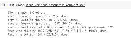
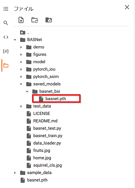
- 学習済みモデルのダウンロード
公式ページ https://github.com/xuebinqin/BASNet の指示による。 学習済みモデル(ファイル名 basenet.pth)は、次で公開されている。 ダウンロードし、saved_models/basnet_bsi の下に置く
https://drive.google.com/open?id=1s52ek_4YTDRt_EOkx1FS53u-vJa0c4nu
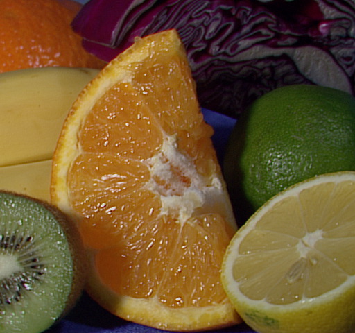
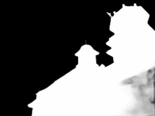
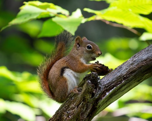
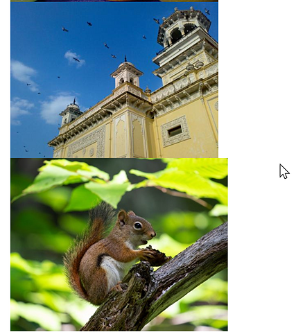
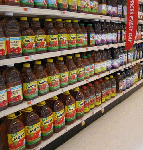
- テスト用の画像のダウンロードと確認表示
%cd BASNet
!curl -L https://github.com/opencv/opencv/blob/master/samples/data/fruits.jpg?raw=true -o fruits.jpg
!curl -L https://github.com/opencv/opencv/blob/master/samples/data/home.jpg?raw=true -o home.jpg
!curl -L https://github.com/opencv/opencv/blob/master/samples/data/squirrel_cls.jpg?raw=true -o squirrel_cls.jpg
from PIL import Image
Image.open('fruits.jpg').show()
Image.open('home.jpg').show()
Image.open('squirrel_cls.jpg').show()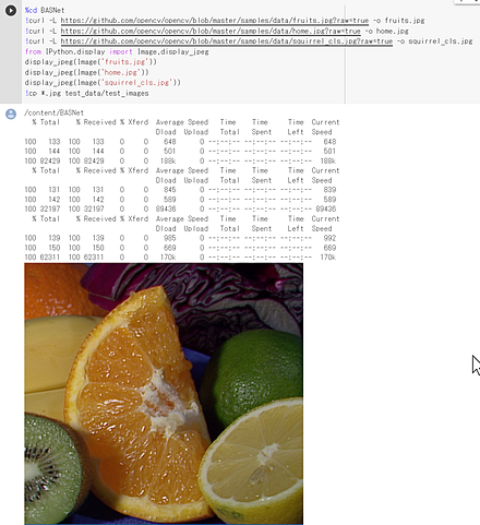
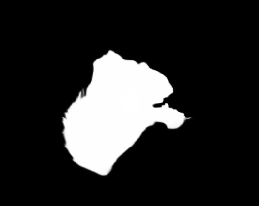
- BASNet の実行
%cd BASNet
!python basnet_test.py
- 結果の表示
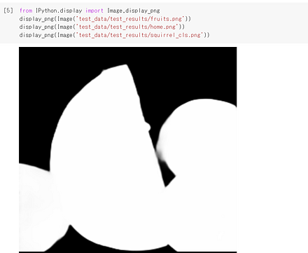
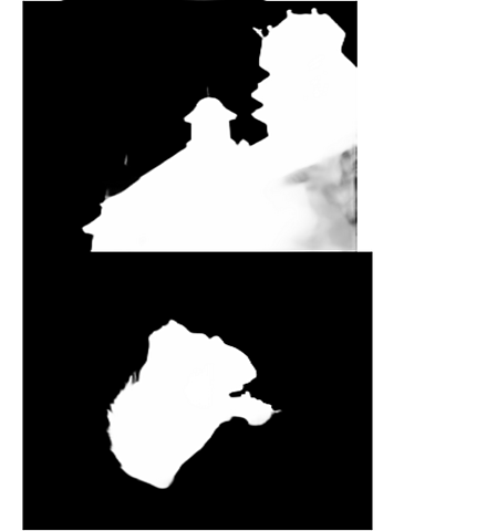
BDD100K
物体検出, instance segmentation, multi object tracking, segmentation tracking, セマンティック・セグメンテーション (semantic segmentation), lane marking, pose estimation 等の用途を想定したデータセット
- 文献 Yu, Fisher and Chen, Haofeng and Wang, Xin and Xian, Wenqi and Chen, Yingying and Liu, Fangchen and Madhavan, Vashisht and Darrell, Trevor, BDD100K: A Diverse Driving Dataset for Heterogeneous Multitask Learning, The IEEE Conference on Computer Vision and Pattern Recognition (CVPR), 2020.
- 公式ページ: https://www.vis.xyz/bdd100k/
- 公式のドキュメント: https://doc.bdd100k.com/usage.html
- BDD100K のダウンロードの公式ページ: https://doc.bdd100k.com/download.html
- 公式の Model Zoo: https://github.com/SysCV/bdd100k-models/
- Papers with Code のページ: https://paperswithcode.com/dataset/bdd100k
【関連項目】 物体検出, instance segmentation, multi object tracking, segmentation tracking, セマンティック・セグメンテーション (semantic segmentation), lane marking, pose estimation
Big Tranfer ResNetV2
【関連項目】 Residual Networks (ResNets)
BioID 顔データベース (BioID Face Database)
BioID 顔データベースは、23名, 1521枚のモノクロの画像。解像度は 384x286 である。目の位置に関するデータを含む。
BioID 顔データベースは次の URL で公開されているデータセット(オープンデータ)である。
BM3D image denosing
BM3D image denosing の公式ソースコード(GitHub のページ): https://github.com/gfacciol/bm3d
【関連項目】 image denosing
Boston housing price 回帰データセット
Boston housing price 回帰データセットは、次のプログラムでロードできる。
from tensorflow.keras.datasets import boston_housing
(x_train, y_train), (x_test, y_test) = boston_housing.load_data()
【関連項目】 Keras に付属のデータセット
Box Annotation
ディープラーニングによる物体検出のための学習と検証では、 アノテーションとして、物体のバウンディングボックスが広く用いられている。
ディープラーニングによるインスタンス・セグメンテーション (instance segmentation)でも、 Tian らの BoxInst (2021年発表) のように、画素単位でのアノテーションでなく、 バウンディングボックスを用いる手法が登場している。
- 文献, Zhi Tian, Chunhua Shen, Xinlong Wang and Hao Chen, BoxInst: High-Performance Instance Segmentation with Box Annotations, CVPR 2021, also CoRR, abs/2012.02310, 2021.
【関連項目】 インスタンス・セグメンテーション (instance segmentation), バウンディングボックス, 物体検出,
cabani の MaskedFace-Net データセット
正しくマスクが装着された状態の顔の写真 (CMFD) と、 正しくマスクが装着されていない状態の顔の写真 (IMFD) のデータセット。
- CMDD: 67,049 枚, 1024x1024
- IMFD: 66,734 枚, 1024x1024
文献
Adnane Cabani and Karim Hammoudi and Halim Benhabiles and Mahmoud Melkemi, MaskedFace-Net -- A Dataset of Correctly/Incorrectly Masked Face Images in the Context of COVID-19, Smart Health, 2020.
Science Direct: https://www.sciencedirect.com/science/article/pii/S2352648320300362
【サイト内の関連ページ】
chandrikadeb7 / Face-Mask-Detection のインストールと動作確認(マスク有り顔、マスクなし顔の検出)(Python、TensorFlow を使用)(Windows 上): 別ページ »で説明
【関連する外部ページ】
公式 URL: https://github.com/cabani/MaskedFace-Net
【関連項目】 顔のデータベース, 顔検出 (face detection)
Caffe
- Caffe の URL: http://caffe.berkeleyvision.org/
Caffe2
【関連する外部ページ】
- URL: https://caffe2.ai
- github: https://github.com/caffe2/caffe2
- モデル zoo: https://caffe2.ai/docs/zoo.html https://github.com/caffe2/models
Caltech Pedestrian データセット (Caltech Pedestrian Dataset)
Caltech Pedestrian データセット は、都市部を走行中の車両から撮影したデータ。 機械学習による物体検出 の学習や検証に利用できるデータセットである。
- 640x480 30Hzのビデオ
- 約10時間分(約25万フレーム、約1分間のセグメントが137個)
- バウンディングボックス: 約35万個、約 2300人の歩行者がアノテーションされている。
- アノテーションは、バウンディングボックスの時間的な対応関係、オクルージョンラベルを含む
Caltech Pedestrian データセットは次の URL で公開されているデータセット(オープンデータ)である。
URL: http://www.vision.caltech.edu/datasets/
【関連情報】
- Papers With Code の Caltech Pedestrian データセットのページ: https://paperswithcode.com/dataset/caltech-pedestrian-dataset
- PyTorch の Caltech Pedestrian データセット: https://pytorch.org/vision/stable/datasets.html#caltech
CSAILVision
CSAILVisionは、Places365データセットを用いた事前学習済みモデルと、それを利用した画像分類、image tagging、Class Activation Mapping (CAM) のプログラムを提供している。
- CSAILVision の Places365
Places365 データセットを用いた事前学習済みモデルと、 それを利用した、画像分類、image tagging、Class Activation Mapping (CAM) のプログラムが公開されている。
【関連項目】 画像分類、 Class Activation Mapping (CAM)、 image tagging
CelebA (Large-scale CelebFaces Attributes) データセットのダウンロード
Large-scale CelebFaces Attributes (CelebA) データセットは、顔画像とアノテーションのデータである。 機械学習による顔検出、顔ランドマーク (facial landmark)、顔認識、顔の生成などの学習や検証に利用できるデータセットである。
- 20万人以上の有名人の画像に、40の属性アノテーションを付けたもの
- 人数: 10,177
- 顔画像: サイズ 178×218 で、202,599枚
- 5つの顔ランドマーク
- 40の属性アノテーション(髪の色、性別、年齢などの顔属性)
Large-scale CelebFaces Attributes (CelebA) データセットは次の URL で公開されているデータセット(オープンデータ)である。
URL: https://mmlab.ie.cuhk.edu.hk/projects/CelebA.html
【関連情報】
- 文献
Deep Learning Face Attributes in the Wild, Ziwei Liu, Ping Luo, Xiaogang Wang, Xiaoou Tang, ICCV 2015.
- Papers With Code の CelebA データセットのページ: https://paperswithcode.com/dataset/celeba
- PyTorch の CelebA データセット: https://pytorch.org/vision/stable/datasets.html#torchvision.datasets.CelebA
- TensorFlow データセット の CelebA データセット: https://www.tensorflow.org/datasets/catalog/celeb_a
【関連項目】 顔のデータベース、顔ランドマーク (facial landmark)
Chain of Thought
マルチモーダル名前付きエンティティ認識(Multimodal Named Entity Recognition; MNER)およびマルチモーダル関係抽出(Multimodal Relation Extraction; MRE)の改善に注力し、これらの分野における精度向上を目指している。この目的のために、Chain of Thought(CoT)プロンプトを活用し、大規模言語モデル(LLM)から reasoning を抽出している。論文の手法は、名詞、文、マルチモーダルの観点からの多粒度の推論と、スタイル、エンティティ、画像を含むデータ拡張を網羅している。これにより、LLMからの reasoning をより効果的に抽出している。MNERの有効性を評価するために、Twitter2015、Twitter2017、SNAP、WikiDiverseという様々なデータセットを使用し、提案方法の効果を検証している。
【文献】
Feng Chen, Yujian Feng, Chain-of-Thought Prompt Distillation for Multimodal Named Entity Recognition and Multimodal Relation Extraction, arXiv:2306.14122v3, 2023.
https://arxiv.org/pdf/2306.14122v3.pdf
【関連する外部ページ】
- LangChain の GitHub のページ: https://github.com/langchain-ai/langchain
- LangChain の公式ドキュメント: https://python.langchain.com/v0.2/docs/introduction/
- LangChain の Paper with Code のページ: https://paperswithcode.com/paper/chain-of-thought-prompt-distillation-for
Chandrika Deb の顔マスク検出 (Chandrika Deb's Face Mask Detection) および顔のデータセット
写真やビデオから、マスクありの顔と、マスク無しの顔を検出する技術およびソフトウェアである。顔検出、マスク有りの顔とマスク無しの顔の分類を同時に行っている。MobileNetV2(ディープニューラルネットワーク)を使用している。
ソースコードは公開されており、画像を追加して学習をやり直すことも可能である。
Bing Search API、Kaggle dataset、RMDF dataset から収集された顔のデータセット(マスクあり: 2165 枚、マスクなし 1930 枚)が同封されている。
【関連する外部ページ】
- GitHub のページ: Chandrika Deb, https://github.com/chandrikadeb7/Face-Mask-Detection
- 正しくマスクをつけた顔と、正しくマスクをつけていない顔のデータセット: https://github.com/cabani/MaskedFace-Net
【関連項目】 cabani の MaskedFace-Net データセット、 Face Mask Detection、 マスク付き顔の処理、 顔検出 (face detection)
Chaudhury らの画像補正 (image rectification)
画像補正は、画像を射影変換することにより、斜め方向からの撮影画像を正面画像に変換する技術である。 意図しないカメラ回転(ロール、ピッチ、ヨー)を含む画像を正面画像に補正できる。
また、AIの事前学習は、通常、正面画像で行われることが多く、画像補正を使うことで、AIの推論をより精度よく行うことができると期待できる。
【文献】
Chaudhury, Krishnendu, Stephen DiVerdi, and Sergey Ioffe. "Auto-rectification of user photos." 2014 IEEE International Conference on Image Processing (ICIP). IEEE, 2014.
【資料】 PDFファイル、パワーポイントファイル
【サイト内の関連ページ】
【関連する外部ページ】
GitHub のページ: https://github.com/chsasank/Image-Rectification
CIFAR-10 データセット
CIFAR-10 データセット(Canadian Institute for Advanced Research, 10 classes)は、公開されているデータセット(オープンデータ)である。
CIFAR-10 データセット(Canadian Institute for Advanced Research, 10 classes) は、クラス数 10 の カラー画像と、各画像に付いたラベルから構成されるデータセットである。 機械学習での画像分類の学習や検証に利用できる。
CIFAR-100 データセット
Cityscapes データセット
Class Activation Mapping (CAM)
Class Activation Mapping (CAM) は、 Bolei Zhou により、2016年に提案された。
- Bolei Zhou らの文献
Bolei Zhou Aditya Khosla Agata Lapedriza Aude Oliva Antonio Torralba, Learning Deep Features for Discriminative Localization, CVPR 2016, also CoRR, https://arxiv.org/abs/1512.04150v1, 2016.
- Bolei Zhou によるソースコードとモデル: https://github.com/zhoubolei/CAM
- Papers with Code のページ: https://paperswithcode.com/paper/learning-deep-features-for-discriminative
【関連項目】 CSAILVision
CRAFT
CRAFT は、文字検出の一手法。
【文献】 Youngmin Baek, Bado Lee, Dongyoon Han, Sangdoo Yun, and Hwalsuk Lee, Character Region Awareness for Text Detection, Proceedings of the IEEE Conference on Computer Vision and Pattern Recognition, pp. 9365--9374, 2019.
【関連する外部ページ】
GitHub のページ: https://github.com/clovaai/CRAFT-pytorch
【関連項目】 EasyOCR
CREPE
CREPE(Convolutional Representation for Pitch Estimation)は、深層学習を用いたモノフォニック音声のピッチ推定手法である。以下に、CREPEの特徴と性能評価について説明する。
特徴
- CREPEは、時間領域の音声波形を直接入力とし、畳み込みニューラルネットワーク(CNN)を用いて360次元のピッチアクティベーションを出力する。
- ピッチアクティベーションは、6オクターブの音域を20セント間隔で分割した360個の音高候補に対する活性度を表す数値ベクトルである。
性能評価
- RWC-synthとMDB-stem-synthの2つのデータセットを用いて、従来手法であるpYINやSWIPEとの比較が行われた。
- 評価指標として、Raw Pitch Accuracy(RPA)とRaw Chroma Accuracy(RCA)が用いられた。
- ピッチ認識の閾値を変化させた場合や、ホワイトノイズ等を加えた場合のロバスト性も評価された。
- 実験の結果、CREPEは多様な音色やノイズに対して従来手法よりもロバスト性に優れ、高精度なピッチ推定が可能であることが示された。
応用分野
- CREPEは、旋律抽出やイントネーション分析など、ピッチ情報を必要とする様々な音声処理タスクに応用可能である。
- 音楽情報処理における音高推定や、言語学における韻律分析などにも活用できる。
文献
CREPE: A Convolutional Representation for Pitch Estimation Jong Wook Kim, Justin Salamon, Peter Li, Juan Pablo Bello. Proceedings of the IEEE International Conference on Acoustics, Speech, and Signal Processing (ICASSP), also arXiv:1802.06182v1 [eess.AS], 2018.
https://arxiv.org/pdf/1802.06182v1
CREPE の GitHub の公式ページ: https://github.com/marl/crepe
【サイト内の関連ページ】 CREPE のインストール、CREPE を用いた音声分析プログラム(音のピッチ推定)(Python、TensorFlow を使用)(Windows 上)
crowd counting (群衆の数のカウントと位置の把握)
crowd countingは、 画像内の人数を数えること。 監視等に役立つ。 さまざま状況において、 さまざまな大きさで画像内にある人物を数えることが課題であり、 画像からの物体検出とは研究課題が異なる。
【関連項目】 FIDTM, JHU-CROWD++ データセット, NWPU-Crowd データセット, ShanghaiTech データセット, UCF-QNRF データセット
CLIP
CLIP(Contrastive Language-Image Pre-Training)では、 テキスト画像のペアを用いて学習が行われる。 GPT-2、GPT-3 のゼロショット学習 (zero-shot learning) のゼロショットと同様に、 画像に対して、テキストが結果として求まる。 CLIP は、ImageNet データセット のゼロショットに対して、 ResNet50と同等の性能があるとされる。
CLIP の GitHub のページ: https://github.com/openai/CLIP
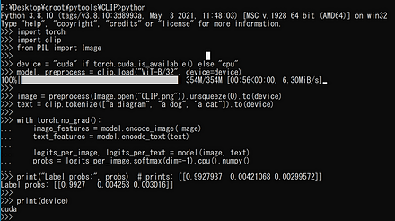
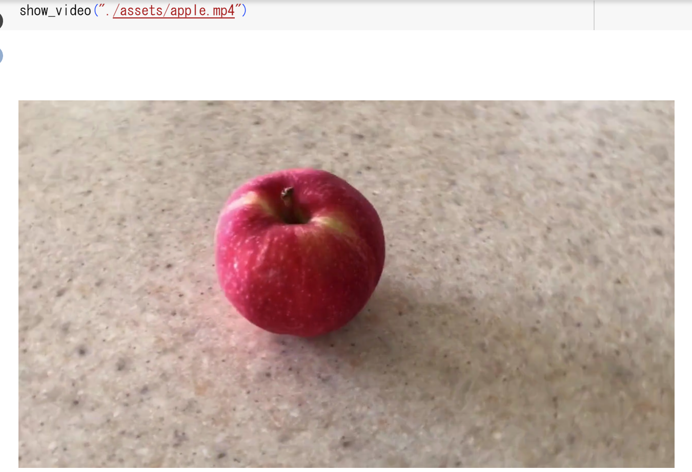
CLIP のサンプルプログラムの実行結果は次の通り。
【関連項目】 AltCLIP
C-MS-Celeb Cleaned データセット
C-MS-Celeb Cleaned データセット は、 MS-Celeb-1M データセット を整えたもの。間違いの修正など。
人物数は 94,682 (94,682 identities), 画像数は 6,464,018 枚 (6,464,018 images)
次の URL で公開されているデータセット(オープンデータ)である。
https://github.com/EB-Dodo/C-MS-Celeb
- 文献
Chi Jin, Ruochun Jin, Kai Chen, and Yong Dou, "A Community Detection Approach to Cleaning Extremely Large Face Database," Computational Intelligence and Neuroscience, vol. 2018, Article ID 4512473, 10 pages, 2018. doi:10.1155/2018/4512473
【関連項目】 顔のデータベース, MS-Celeb-1M データセット, 顔検出 (face detection)
CNN
CNN (convolutional neural network) は畳み込みニューラルネットワークのこと。
CNTK
- Web ページ:
https://github.com/microsoft/CNTK - github: https://github.com/Microsoft/CNTK
- チュートリアル: http://research.microsoft.com/en-us/um/people/dongyu/CNTK-Tutorial-NIPS2015.pdf
- ドキュメント: http://research.microsoft.com/apps/pubs/?id=226641
- ChainerCV について: https://github.com/chainer/chainercv
- Python について: https://github.com/stitchfix/Algorithms-Notebooks
COCO (Common Object in Context) データセット
COCO の Keypoints 2014/2017 アノテーション
URL: https://cocodataset.org/#keypoints-2017
COCO の Keypoints 2014/2017 アノテーションは、次からダウンロードできる。
- https://drive.google.com/file/d/1jrxis4ujrLlkwoD2GOdv3PGzygpQ04k7/view
- https://drive.google.com/file/d/1YuzpScAfzemwZqUuZBrbBZdoplXEqUse/view
COLMAP
COLMAP は 3次元再構成の機能を持ったソフトウェア。
【文献】
Johannes L. Schonberger, Jan-Michael Frahm, Structure-From-Motion Revisited, CVPR 2016, 2016
【サイト内の関連ページ】
- COLMAP 3.8 のインストールと3次元再構成の実行(COLMAP 3.8 を使用)(Windows 上): 別ページ »で説明
- COLMAP のインストールと3次元再構成の実行(COLMAP のソースコード、vcpkgm, Visual Studio Community 2019 を使用)(Windows 上): 別ページ »で説明
【関連する外部ページ】
- Papers with Code の colmap のページ: https://paperswithcode.com/paper/structure-from-motion-revisited
- COLMAP の公式ページ(公式リリース、Vocabulary tree, データセットへのリンクなど): https://demuc.de/colmap
- COLMAP の公式の説明: https://colmap.github.io
- COLMAP を公開している公式ページ: https://github.com/colmap/colmap/releases
- Gerrard Hall, Craham Hall, Person Hall, South Building データセット: https://colmap.github.io/datasets.html
Coqui TTS
Coqui TTS は、音声合成および音声変換(Voice Changer)の研究プロジェクトならびに成果物。
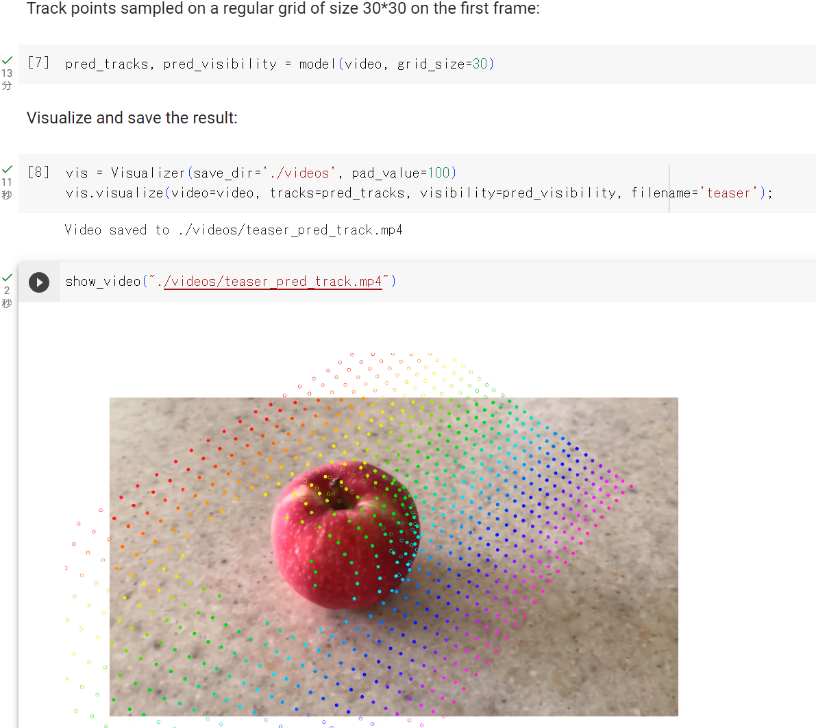
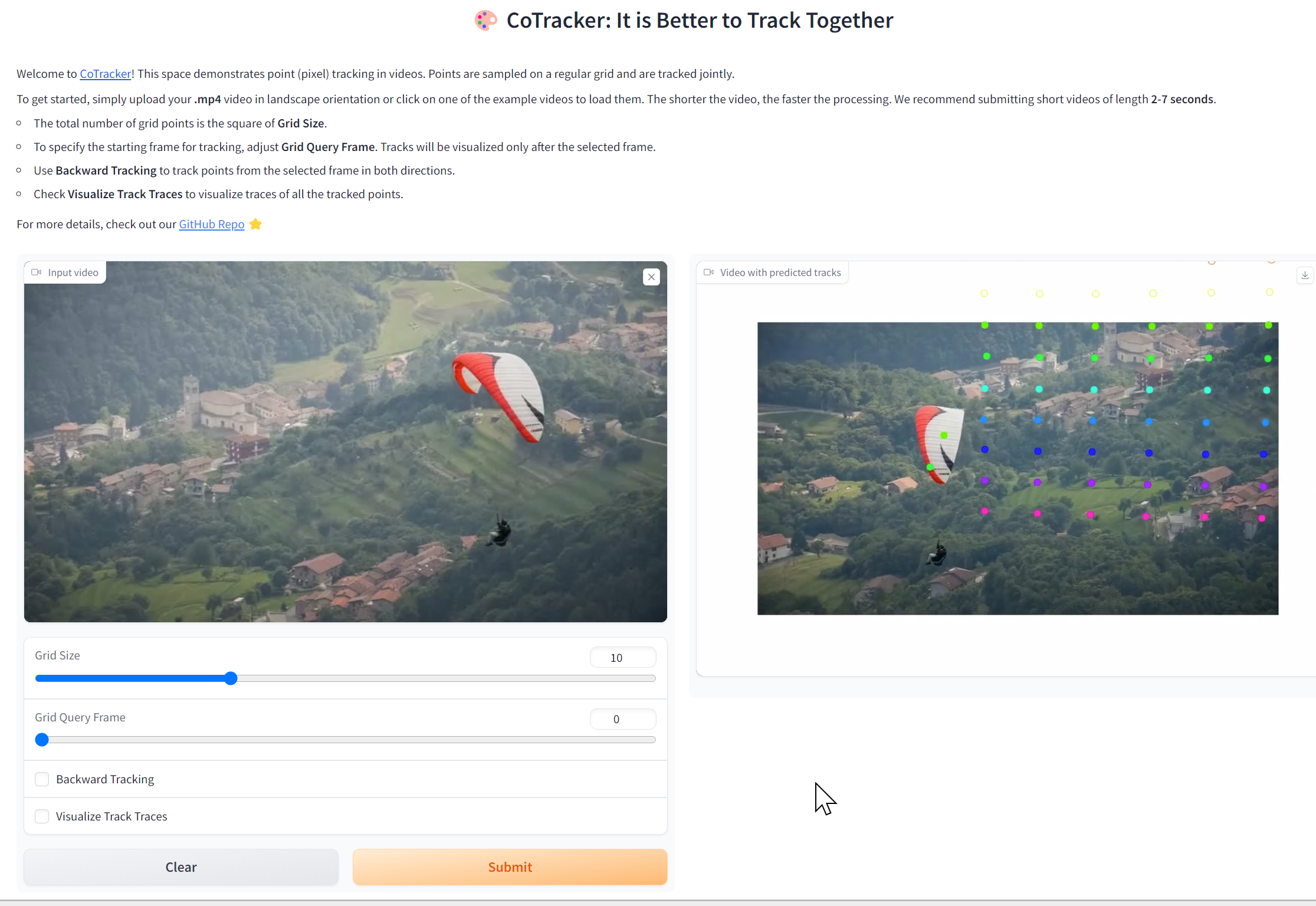
CoTracker
CoTracker は、動画のポイントトラッキングの一手法である。 この手法は、長期間の追跡やオクルージョン(遮蔽)の取り扱いの難しさに対処するために開発された。 CoTracker では、ポイントをグループとして追跡する方法、つまりグループベースのアプローチを採用しており、ポイント間の相互関係を活用する。さらに、時間的なスライディングウィンドウメカニズムを使用して、長期間にわたる追跡を行う。実験結果からは、co-trackingが既存の手法に比べて、オクルージョンや長期間のビデオに対する追跡の安定性が向上したことが示されている。
【文献】
Nikita Karaev, Ignacio Rocco, Benjamin Graham, Natalia Neverova, Andrea Vedaldi, Christian Rupprecht, CoTracker: It is Better to Track Together, arXiv:2307.07635v1, 2023.
https://arxiv.org/pdf/2307.07635v1.pdf
【関連する外部ページ】
- CoTracker のデモ(Google Colaboratory)
- CoTracker の Hugging Face のデモ
https://huggingface.co/spaces/facebook/cotracker
- GitHub のページ: https://github.com/facebookresearch/co-tracker
- Paper with Code のページ: https://paperswithcode.com/paper/cotracker-it-is-better-to-track-together
CSPNet (Cross Stage Parital Network)
CSPNet は、ステージの最初の特徴マップ (feature map) と最後の特徴マップ (feature map) を統合することを特徴とする手法。
CSPNet は、 ResNet, ResNeXt, DenseNet などに適用でき、 ImageNet データセットを用いた画像分類の実験では、計算コスト、メモリ使用量、推論の速度、推論の精度の向上ができるとされている。 その結果として、物体検出 についても改善ができるとされている。
CSPNet の公式の実装 (GitHub) のページでは、 画像分類として、 CSPDarkNet-53、 CSPResNet50、 CSPResNeXt-50, 物体検出として、 CSPDarknet53-PANet-SPP, CSPResNet50-PANet-SPP, CSPResNeXt50-PANet-SPP 等の実装が公開されている。
Scaled YOLO v4 では、CSPNet の技術が使われている。
- 文献
Chien-Yao Wang, Hong-Yuan Mark Liao, I-Hau Yeh, Yueh-Hua Wu, Ping-Yang Chen, Jun-Wei Hsieh, CSPNet: A New Backbone that can Enhance Learning Capability of CNN, CoRR, abs/1911.11929v1, 2019.
- CSPNet の公式の実装 (GitHub) のページ: https://github.com/WongKinYiu/CrossStagePartialNetworks
- Ross Wightman の pytorch-image-models (GitHub) のページ: https://github.com/rwightman/pytorch-image-models
【関連項目】 AlexeyAB darknet, 画像分類, 物体検出, Scaled YOLO v4, pytorchimagemodels
CSAILVision
CSAILVision の公式デモ(GitHub のページ): https://colab.research.google.com/github/CSAILVision/semantic-segmentation-pytorch/blob/master/notebooks/DemoSegmenter.ipynb
【関連項目】 セマンティックセグメンテーション (semantic segmentation)
CuPy
CuPy は NumPyのGPU実装であり、CUDA対応GPUで高速な数値計算を行うためのPythonライブラリである。
【関連する外部ページ】
- CuPy の公式ページ: https://cupy.chainer.org/
- CuPy の公式のインストールページ: https://docs.cupy.dev/en/stable/install.html
【サイト内の関連ページ】
- CuPy 13.2 のインストール、CuPy のプログラム例(Windows 上): 別ページ »で説明
【関連項目】 NVIDIA CUDA
CuRRET データベース (Columbia-Utrecht Reflectance and Texture Database)
反射率とテクスチャに関するデータベース
- BRDF データベース: 60 以上のサンプルについて、反射率を計測したもの。
- BRDF パラメータデータベース: BRDF モデル(the Oren-Nayar model とthe Koenderink et al. representation の2つ)のフィッティングパラメータ (fitting parameter) を含む。
- BTF データベース: 60 以上のサンプルについての画像テクスチャに関する計測値
CuRRET データベース (Columbia-Utrecht Reflectance and Texture Database)は次の URL で公開されているデータセット(オープンデータ)である。
URL: https://www.cs.columbia.edu/CAVE/software/curet/html/about.php
DeepFace
DeepFace は、ArcFace 法による顔識別の機能や、顔検出、年齢や性別や表情の推定の機能などを持つ。
ArcFace 法は、距離学習の技術の1つである。 画像分類において、種類が不定個であるような画像分類に使うことができる技術である。 顔のみで動くということではないし、 顔の特徴を捉えて工夫されているということもない。
DeepFace の URL: https://github.com/serengil/deepface
ArcFace 法の概要は次の通り
- 顔のコード化:顔画像を、数値ベクトル(数値の並び)に変換する。
- 顔のコードについて、同一人物の顔のコードは近くになるように、違う人物の顔のコードは遠くなるように、顔のコードを作り直す。そのときディープラーニングを使う。これを「距離学習」という。
- 距離学習の学習済みモデルを使う。距離学習がなかったときと比べて、顔認識の精度の向上が期待できる。
【関連項目】 ArcFace 法, 顔検出, 顔識別 (face identification), 顔認識, 顔に関する処理
DeepForge
DeepForge は,ディープラーニングのソフトウェア一式である.Webサーバも付属しており,Webブラウザからディープラーニングのソフトウェアの作成,実行,保存が簡単にできる.ソフトウェアの作成は,Webブラウザ上でのエディタでも,Webブラウザ上でのビジュアルなエディタでもできる.ディープラーニングでのニューラルネットワークの構造が図で簡単に確認できて便利である.
【サイト内の関連ページ】
- Windows での DeepForge のインストールとテスト実行: 別ページで説明している.
【関連する外部ページ】
- DeepForge の公式ページ: https://deepforge.org/
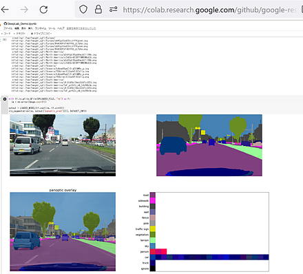
DeepLab2
DeepLab2 は,セグメンテーションの機能を持つ TensorFlow のライブラリである. DeepLab, Panoptic-DeepLab, Axial-DeepLab, Max-DeepLab, Motion-DeepLab, ViP-DeepLab を含む.
DeepLab2 の公式のデモ(Google Colaboratory のページ)の実行により,下図のように panoptic segmentation の結果が表示される.
そのデモのページの URL: https://colab.research.google.com/github/google-research/deeplab2/blob/main/DeepLab_Demo.ipynb#scrollTo=6552FXlAOHnX
【文献】
Mark Weber, Huiyu Wang, Siyuan Qiao, Jun Xie, Maxwell D. Collins, Yukun Zhu, Liangzhe Yuan, Dahun Kim, Qihang Yu, Daniel Cremers, Laura Leal-Taixe, Alan L. Yuille, Florian Schroff, Hartwig Adam, Liang-Chieh Chen, DeepLab2: A TensorFlow Library for Deep Labeling, CoRR, abs/2106.09748v1, 2021.
【サイト内の関連ページ】
Windows で動く人工知能関係 Pythonアプリケーション,オープンソースソフトウエア: 別ページ »で説明している.
【関連する外部ページ】
- https://arxiv.org/pdf/2106.09748v1.pdf
- DeepLab2 の GitHub のページ: https://github.com/google-research/deeplab2
- DeepLab2 の Google Colaboratory のページ: https://colab.research.google.com/github/google-research/deeplab2/blob/main/DeepLab_Demo.ipynb
【関連項目】 セマンティック・セグメンテーション (semantic segmentation), panoptic segmentation, depth estimation
DeepLab2 のインストール(Windows 上)
- プロトコル・バッファ・コンパイラ (protocol buffer compiler) のインストールを行っておく.
- コマンドプロンプトを管理者として開く.
- DeepLab2 のダウンロード,前提ソフトウエアのインストール
DeepLab2 を動かすため,protobuf==3.19.6 を指定する.
cd c:\ rmdir /s /q c:\deeplab2 mkdir c:\deeplab2 cd c:\deeplab2 git clone https://github.com/google-research/deeplab2.git python -m pip install -U tensorflow==2.10.1 protobuf==3.19.6 - protoc を用いてコンパイル
cd c:\deeplab2
protoc deeplab2\*.proto --python_out=.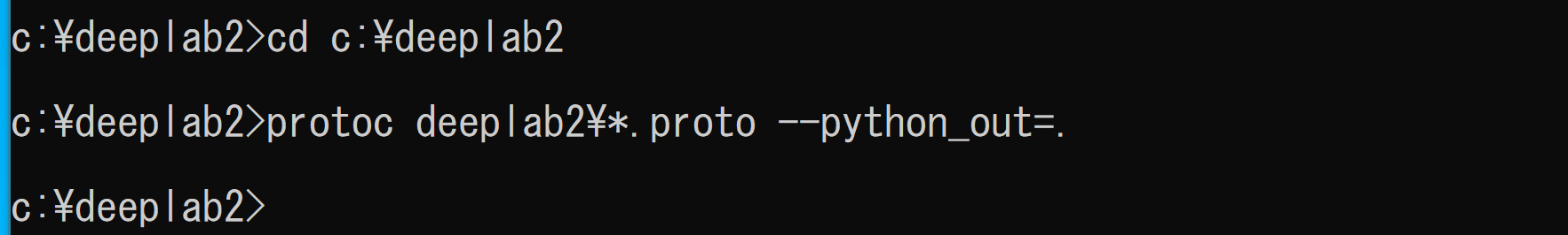
- Windows の システム環境変数 PYTHONPATHに,c:\deeplab2 を追加することにより,パスを通す.
Windows で,管理者権限でコマンドプロンプトを起動(手順:Windowsキーまたはスタートメニュー >
cmdと入力 > 右クリック > 「管理者として実行」).powershell -command "$oldpath = [System.Environment]::GetEnvironmentVariable(\"PYTHONPATH\", \"Machine\"); $oldpath += \";c:\deeplab2\"; [System.Environment]::SetEnvironmentVariable(\"PYTHONPATH\", $oldpath, \"Machine\")"
- 新しくコマンドプロンプトを開き,動作確認
cd c:\deeplab2\deeplab2\model
python deeplab_test.py
DeepLab2 のインストール(Ubuntu 上)
https://github.com/google-research/deeplab2/blob/main/g3doc/setup/installation.md の記載による.
- protoc のインストール
# パッケージリストの情報を更新 sudo apt update sudo apt -y install libprotobuf-dev protobuf-compiler protobuf-c-compiler python3-protobuf - pycocotools のインストール
sudo pip3 install tensorflow tf-models-official pillow matplotlib cython sudo pip3 install "git+https://github.com/philferriere/cocoapi.git#egg=pycocotools&subdirectory=PythonAPI" # install pycocotools cd /usr/local sudo git clone https://github.com/cocodataset/cocoapi.git sudo chown -R $USER cocoapi cd ./cocoapi/PythonAPI make echo 'export PYTHONPATH=$PYTHONPATH:/usr/local/cocoapi/PythonAPI' >> ~/.bashrc - DeepLab2 のインストール
cd /usr/local sudo rm -rf deeplab2 sudo git clone https://github.com/google-research/deeplab2.git sudo chown -R $USER deeplab2 cd /usr/local protoc deeplab2/*.proto --python_out=. cd /usr/local bash deeplab2/compile.sh echo 'export PYTHONPATH=$PYTHONPATH:/usr/local' >> ~/.bashrc echo 'export PYTHONPATH=$PYTHONPATH:/usr/local/deeplab2' >> ~/.bashrc - TensorFlow モデルのインストール
cd /usr/local sudo rm -rf models sudo git clone https://github.com/tensorflow/models.git sudo chown -R $USER models cd /usr/local/models/research protoc object_detection/protos/*.proto --python_out=. protoc lstm_object_detection/protos/*.proto --python_out=. cd /usr/local/models/research/delf protoc delf/protos/*.proto --python_out=. echo 'export PYTHONPATH=$PYTHONPATH:/usr/local/models' >> ~/.bashrc - DeepLab2 の動作確認
source ~/.bashrc
cd /usr/local
# Model training test (test for custom ops, protobuf)
python deeplab2/model/deeplab_test.py

# Model evaluator test (test for other packages such as orbit, cocoapi, etc)
python deeplab2/trainer/evaluator_test.py
DeepLabv3
セマンティック・セグメンテーションのモデルである. 2017年発表.
- 文献
Liang-Chieh Chen, George Papandreou, Florian Schroff, Hartwig Adam, Rethinking Atrous Convolution for Semantic Image Segmentation
- 公式のソースコード: https://github.com/tensorflow/models/tree/master/research/deeplab
- MMSegmentation の DeepLabv3 のページ: https://github.com/open-mmlab/mmsegmentation/tree/master/configs/deeplabv3
【関連項目】 Residual Networks (ResNets) , モデル, セマンティック・セグメンテーション
DeepLabv3+
セマンティック・セグメンテーションのモデルである. 2018年発表.
- 文献
Liang-Chieh Chen and Yukun Zhu and George Papandreou and Florian Schroff and Hartwig Adam, Encoder-Decoder with Atrous Separable Convolution for Semantic Image Segmentation, ECCV, 2018.
- 公式のソースコード: https://github.com/tensorflow/models/tree/master/research/deeplab
- MMSegmentation の DeepLabv3+ のページ: https://github.com/open-mmlab/mmsegmentation/tree/master/configs/deeplabv3plus
【関連項目】 Residual Networks (ResNets) , モデル, セマンティック・セグメンテーション
DeepXi
- 文献
Nicolson Aaron, Paliwal Kuldip K., Deep Xi as a Front-End for Robust Automatic Speech Recognition, 2020.
- GitHub のページ: https://github.com/anicolson/DeepXi
- Papers with Code のページ: https://paperswithcode.com/paper/deep-xi-as-a-front-end-for-robust-automatic
【関連項目】 speech enhancement, speech recognition
Google Colaboratory での DeepXi のインストール
公式の手順 https://github.com/anicolson/DeepXi による.
次のコマンドやプログラムは Google Colaboratory で動く(コードセルを作り,実行する).
%cd /content
!rm -rf DeepXi
!git clone https://github.com/anicolson/DeepXi.git
%cd DeepXi
!pip3 install -r requirements.txt
Deformable DETR
物体検出の一手法.2021 年発表.
- 文献
Xizhou Zhu and Weijie Su and Lewei Lu and Bin Li and Xiaogang Wang and Jifeng Dai, Deformable DETR: Deformable Transformers for End-to-End Object Detection, International Conference on Learning Representations, also CoRR, abs/2010.04159v4, 2021.
- 公式の URL: https://openreview.net/forum?id=gZ9hCDWe6ke
- 公式のソースコード (GitHub): https://github.com/fundamentalvision/Deformable-DETR
- Papers with Code のページ: https://paperswithcode.com/paper/deformable-detr-deformable-transformers-for-1
- MMDetection のモデル: https://github.com/open-mmlab/mmdetection/blob/master/configs/deformable_detr/README.md
【関連項目】 DETR, MMDetection, 物体検出
Demucs
音源分離(music source separation)を行う一手法.2019年発表.2021年に hybrid version が発表された. 音声と楽器音の混合から,音声や楽器音を分離できる.
- 文献
Hybrid Spectrogram and Waveform Source Separation, Alexandre Défossez, Proceedings of the ISMIR 2021 Workshop on Music Source Separation, also CoRR, abs/2111.03600v1, 2021.
- 公式のページ (GitHub): https://github.com/facebookresearch/demucs
- 公式のオンラインデモ (Google Colaboratory): https://colab.research.google.com/drive/1dC9nVxk3V_VPjUADsnFu8EiT-xnU1tGH?usp=sharing
- 公式のオンラインデモ (HuggingFace 内): https://huggingface.co/spaces/akhaliq/demucs
【関連項目】 audio source separation, music source separation
Google Colaboratory で,音声,楽曲の分離 (Demucs を使用)
公式の手順 https://github.com/facebookresearch/demucs による.
次のコマンドやプログラムは Google Colaboratory で動く(コードセルを作り,実行する).
- Demucs のインストール
!pip3 install -U git+https://github.com/facebookresearch/demucs#egg=demucs
!pip3 show demucs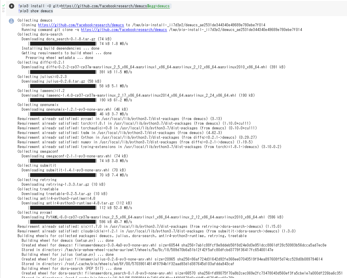
- 処理したいサウンドファイルの準備
ここでは,1.m4a をダウンロードしている.
%cd /content
!curl -O https://www.kkaneko.jp/sample/audio/1.m4a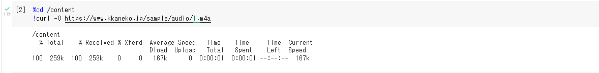
- Demucs の実行
!demucs 1.m4a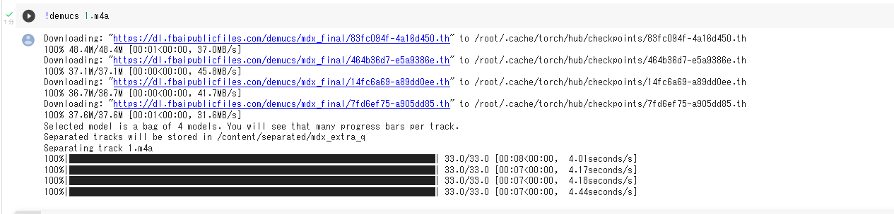
- 処理結果のダウンロード
「1」のところは,処理したサウンドファイルのファイル名にあわせること.
from google.colab import files
%cd separated/mdx_extra_q/1
files.download('drums.wav')
files.download('bass.wav')
files.download('other.wav')
files.download('vocals.wav')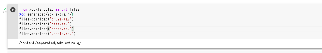
DenseNet121, DenseNet169
CoRR, abs/1608.06993
Keras の DenseNet121 を用いて DenseNet121 を作成するプログラムは次のようになる. 「weights=None」を指定することにより,最初,重みをランダムに設定する.
m = tf.keras.applications.densenet.DenseNet121(input_shape=INPUT_SHAPE, weights=None, classes=NUM_CLASSES)
Keras の DenseNet169 を用いて DenseNet169 を作成するプログラムは次のようになる. 「weights=None」を指定することにより,最初,重みをランダムに設定する.
m = tf.keras.applications.densenet.DenseNet169(input_shape=INPUT_SHAPE, weights=None, classes=NUM_CLASSES)
Keras の応用のページ: https://keras.io/api/applications/
PyTorch, torchvision の DenseNet121 学習済みモデルのロード,画像分類のテスト実行
Google Colab あるいはパソコン(Windows あるいは Linux)を使用.
- 前準備
前準備として,Python のインストール(別項目で説明している), PyTorch のインストール を行う.
Google Colaboratory では, Python, PyTorch はインストール済みなので,インストール操作は不要である.次に,pip を用いて,pillow のインストールを行う.
pip install -U pillow - ImageNet データセット で学習済みのDenseNet121 モデルのロード
PyTorch, torchvision のモデルについては: https://pytorch.org/vision/stable/models.html に説明がある.
import torch import torchvision.models as models device = torch.device('cuda' if torch.cuda.is_available() else 'cpu') m = models.densenet121(pretrained=True).to(device) - 画像分類したい画像ファイルのダウンロードとロードと確認表示
from PIL import Image
import requests

# ダウンロードとロード
url = 'https://github.com/pytorch/hub/raw/master/images/dog.jpg'
response = requests.get(url)
img = Image.open(requests.get(url, stream=True).raw)

# 確認表示
display(img)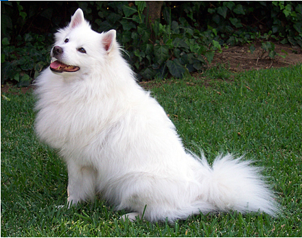
- 画像の前処理.PyTorch で扱えるようにするため.
from PIL import Image from torchvision import transforms img = Image.open(filename) preprocess = transforms.Compose([ transforms.Resize(256), transforms.CenterCrop(224), transforms.ToTensor(), transforms.Normalize(mean=[0.485, 0.456, 0.406], std=[0.229, 0.224, 0.225]), ]) input_tensor = preprocess(img) input_batch = input_tensor.unsqueeze(0) - 推論 (inference) の実行
「m.eval()」は,推論を行うときのためのものである.これを行わないと訓練(学習)が行われる.
import torch if torch.cuda.is_available(): input_batch = input_batch.to('cuda') m.eval() with torch.no_grad(): output = m(input_batch) - 結果の表示
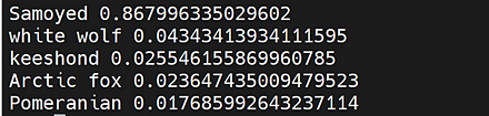
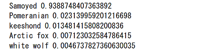
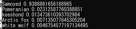
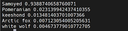
import urllib
url, filename = ("https://raw.githubusercontent.com/pytorch/hub/master/imagenet_classes.txt", "imagenet_classes.txt")
try: urllib.URLopener().retrieve(url, filename)
except: urllib.request.urlretrieve(url, filename)

with open("imagenet_classes.txt", "r") as f:
    categories = [s.strip() for s in f.readlines()]

# The output has unnormalized scores. To get probabilities, you can run a softmax on it.
probabilities = torch.nn.functional.softmax(output[0], dim=0)
print(probabilities)

top5_prob, top5_catid = torch.topk(probabilities, 5)
for i in range(top5_prob.size(0)):
    print(categories[top5_catid[i]], top5_prob[i].item())
Google Colaboratory での結果
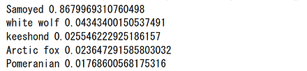
Windows での結果
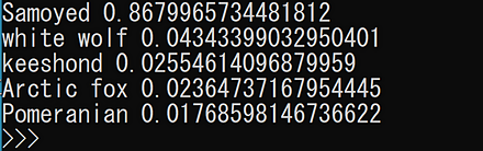
Linux での結果
PyTorch, torchvision の DenseNet169 学習済みモデルのロード,画像分類のテスト実行
Google Colab あるいはパソコン(Windows あるいは Linux)を使用.
- 前準備
前準備として,Python のインストール(別項目で説明している), PyTorch のインストール を行う.
Google Colaboratory では, Python, PyTorch はインストール済みなので,インストール操作は不要である.次に,pip を用いて,pillow のインストールを行う.
pip install -U pillow - ImageNet データセット で学習済みのDenseNet169 モデルのロード
PyTorch, torchvision のモデルについては: https://pytorch.org/vision/stable/models.html に説明がある.
import torch import torchvision.models as models device = torch.device('cuda' if torch.cuda.is_available() else 'cpu') m = models.densenet169(pretrained=True).to(device) - 画像分類したい画像ファイルのダウンロードとロードと確認表示
from PIL import Image
import requests
from IPython.display import display

# ダウンロードとロード
url = 'https://github.com/pytorch/hub/raw/master/images/dog.jpg'
response = requests.get(url)
img = Image.open(requests.get(url, stream=True).raw)

# 確認表示
display(img)
- 画像の前処理.PyTorch で扱えるようにするため.
from PIL import Image from torchvision import transforms img = Image.open(filename) preprocess = transforms.Compose([ transforms.Resize(256), transforms.CenterCrop(224), transforms.ToTensor(), transforms.Normalize(mean=[0.485, 0.456, 0.406], std=[0.229, 0.224, 0.225]), ]) input_tensor = preprocess(img) input_batch = input_tensor.unsqueeze(0) - 推論 (inference) の実行
「m.eval()」は,推論を行うときのためのものである.これを行わないと訓練(学習)が行われる.
import torch if torch.cuda.is_available(): input_batch = input_batch.to('cuda') m.eval() with torch.no_grad(): output = m(input_batch) - 結果の表示
import urllib
url, filename = ("https://raw.githubusercontent.com/pytorch/hub/master/imagenet_classes.txt", "imagenet_classes.txt")
try: urllib.URLopener().retrieve(url, filename)
except: urllib.request.urlretrieve(url, filename)

with open("imagenet_classes.txt", "r") as f:
    categories = [s.strip() for s in f.readlines()]

# The output has unnormalized scores. To get probabilities, you can run a softmax on it.
probabilities = torch.nn.functional.softmax(output[0], dim=0)
print(probabilities)

top5_prob, top5_catid = torch.topk(probabilities, 5)
for i in range(top5_prob.size(0)):
    print(categories[top5_catid[i]], top5_prob[i].item())
Google Colaboratory での結果
Windows での結果
Linux での結果
depth image
depth image は遠近である depth を示す画像である. 画素ごとの色や明るさで depth を表示する.
画像からの depth image の推定は,ステレオカメラや動画から視差を得る方法が主流である.
monodepth2 法
単一のカメラでの画像から depth image を推定する方法としては,ディープラーニングを用いる monodepth2 法 (2019 年発表) が知られる.
monodepth2 の GitHub のページ: https://github.com/nianticlabs/monodepth2
次のコマンドやプログラムは Google Colaboratory で動く(コードセルを作り,実行する).
- インストール
!pip3 install -U numpy pillow matplotlib torch torchvision opencv-python opencv-contrib-python scikit-image
!git clone --recursive https://github.com/nianticlabs/monodepth2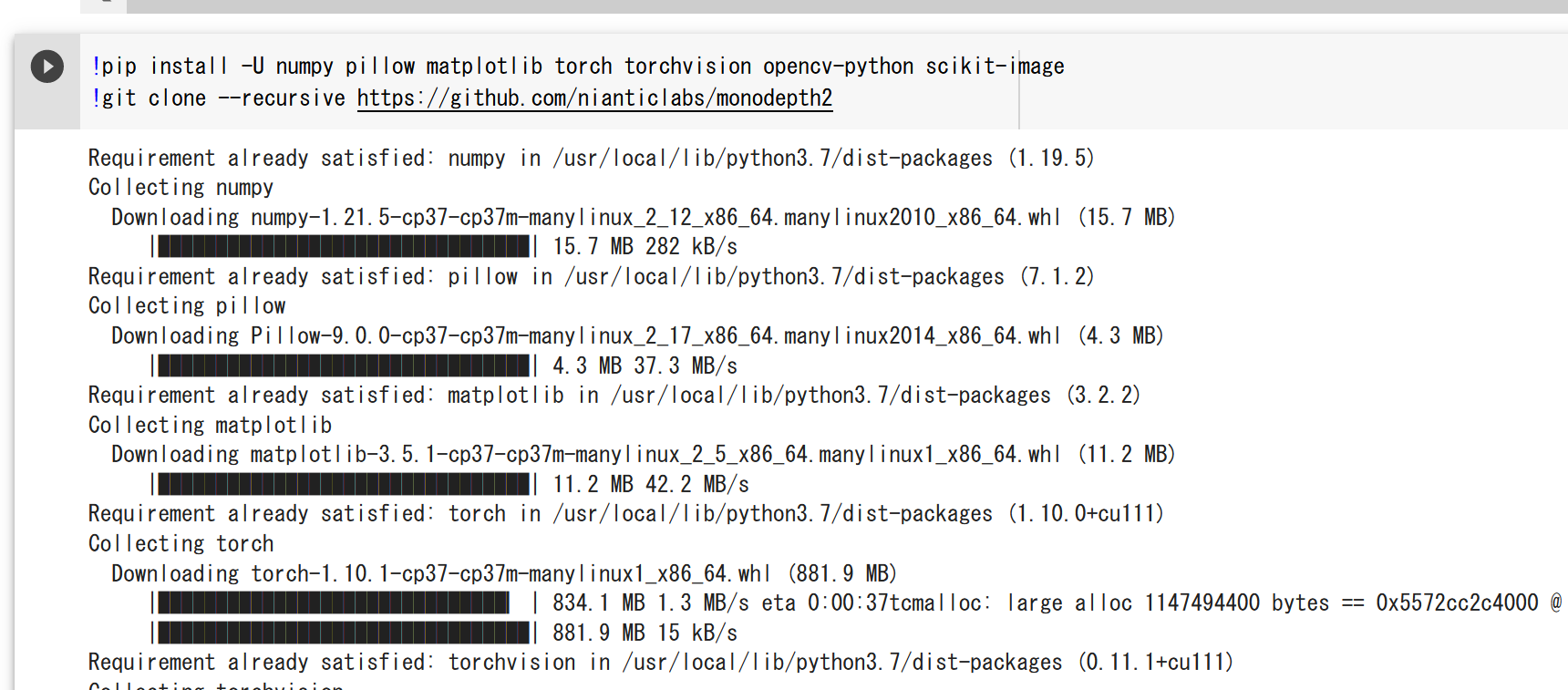
- depth image プログラムの実行
%cd monodepth2
!python3 test_simple.py --image_path assets/test_image.jpg --model_name mono+stereo_640x192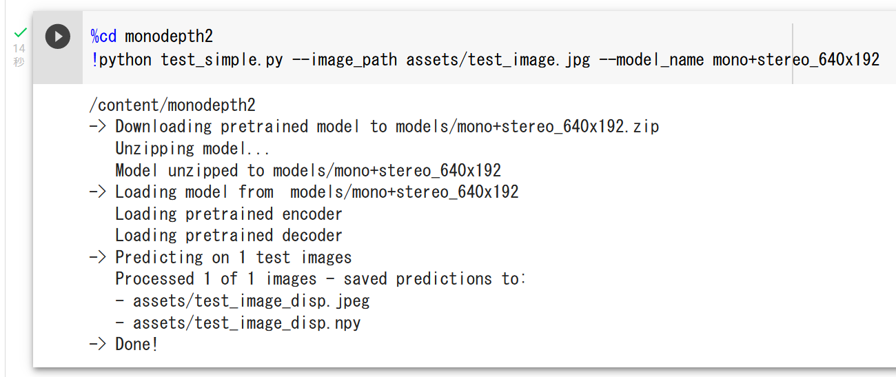
- 画像表示
from PIL import Image
Image.open('assets/test_image.jpg').show()
Image.open('assets/test_image_disp.jpeg').show()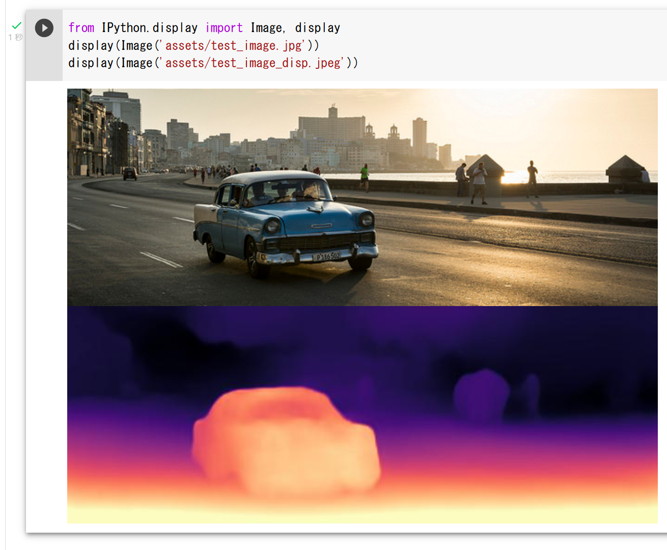
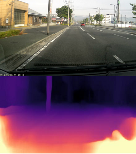
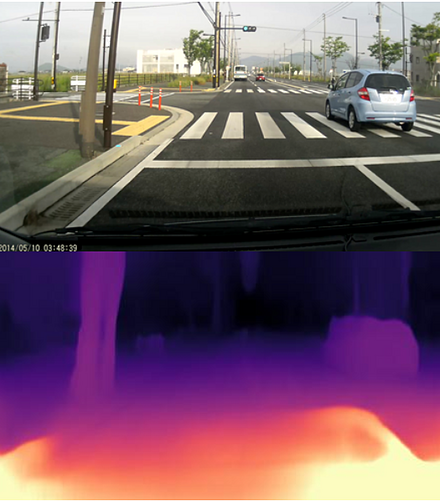
- 他の画像で試した場合
Detectron2
【文献】
Yuxin Wu and Alexander Kirillov and Francisco Massa and Wan-Yen Lo and Ross Girshick, Detectron2, https://github.com/facebookresearch/detectron2, 2019.
【サイト内の関連ページ】
物体検出,インスタンス・セグメンテーション,パノプティック・セグメンテーションの実行(Detectron2,PyTorch, Python を使用)(Windows 上)
【関連する外部ページ】
- GitHub のページ: https://github.com/facebookresearch/detectron2
- ドキュメント: https://detectron2.readthedocs.io/en/latest/tutorials/getting_started.html
- 関連プロジェクトのページ: https://github.com/facebookresearch/detectron2/tree/master/projects
【関連項目】 ADE20K データセット, インスタンス・セグメンテーション (instance segmentation)
Google Colaboratory で,Detectron2 のインスタンス・セグメンテーションの実行
インストールは次のページで説明されている.
https://github.com/facebookresearch/detectron2/releases
次のコマンドやプログラムは Google Colaboratory で動く(コードセルを作り,実行する).
- Google Colaboratory で,ランタイムのタイプを GPU に設定する.
- まず,PyTorch のバージョンを確認する.
PyTorch は,ディープラーニングのフレームワークの機能を持つ Python のパッケージである.
次のプログラム実行により,PyTorch のバージョンが「1.10.0+cu111」のように表示される.
import torch print(torch.__version__) - NVIDIA CUDA ツールキット のバージョンを確認する.
NVIDIA CUDA ツールキットは,NVIDIA社が提供している GPU 用のツールキットである.GPU を用いた演算のプログラム作成や動作のための各種機能を備えている.ディープラーニングでも利用されている.
次のプログラム実行により,NVIDIA CUDA ツールキットのバージョンが「cu111」のように表示される.
import torch
CUDA_VERSION = torch.__version__.split("+")[-1]
print(CUDA_VERSION)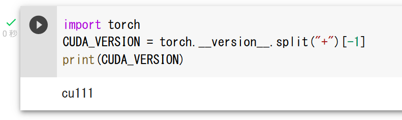
- PyTorch のバージョンを確認する.
import torch
TORCH_VERSION = ".".join(torch.__version__.split(".")[:2])
print(TORCH_VERSION)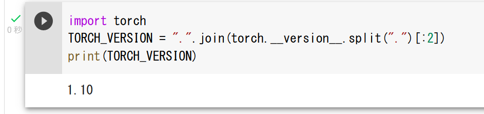
- Detectron2 のインストール
NVIDIA CUDA ツールキット 11.1, PyTorch 1.10 の場合には,次のようになる.
「cu111/torch1.10」のところは, NVIDIA CUDA ツールキット のバージョン, PyTorch のバージョンに合わせる.
!pip3 install detectron2==0.6 -f https://dl.fbaipublicfiles.com/detectron2/wheels/cu111/torch1.10/index.html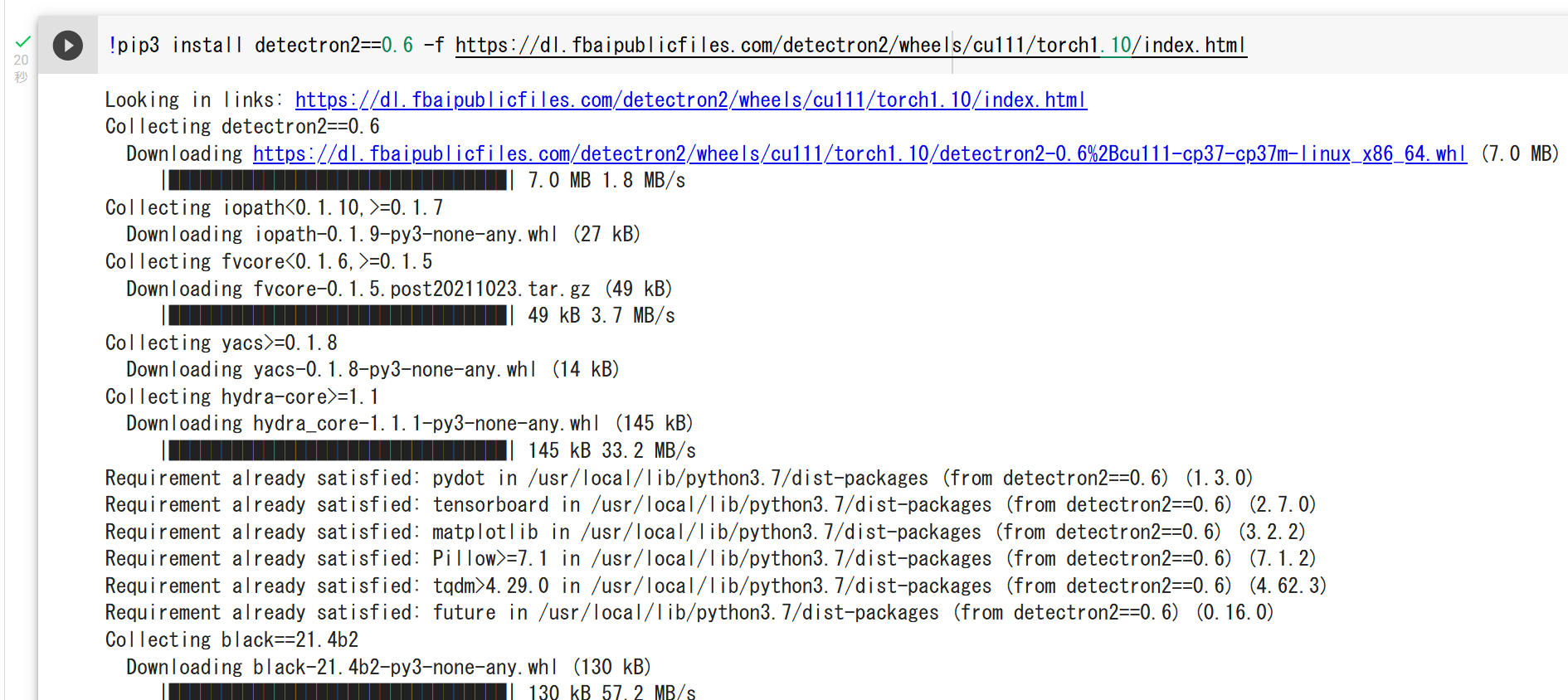
- Detectron2 のソースコードをダウンロード
必要に応じて,中のファイルを利用できるように準備しておく.
!curl -LO https://github.com/facebookresearch/detectron2/archive/refs/tags/v0.6.tar.gz
!tar -xvzof v0.6.tar.gz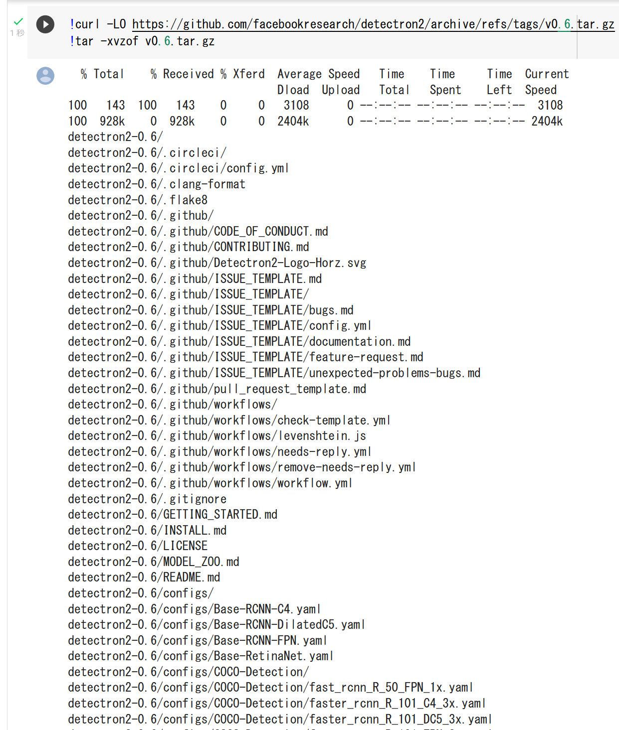
- COCO (Common Objects in Context) データセットの中の画像ファイルをダウンロード
https://colab.research.google.com/drive/16jcaJoc6bCFAQ96jDe2HwtXj7BMD_-m5#scrollTo=FsePPpwZSmqt の記載による.
!curl -O http://images.cocodataset.org/val2017/000000439715.jpg
from PIL import Image
Image.open('000000439715.jpg').show()
- インスタンス・セグメンテーションの実行
https://colab.research.google.com/drive/16jcaJoc6bCFAQ96jDe2HwtXj7BMD_-m5#scrollTo=FsePPpwZSmqt の記載による.
「im = cv2.imread('000000439715.jpg')」で,処理したい画像ファイルをロードしている.
import detectron2
from detectron2 import model_zoo
from detectron2.engine import DefaultPredictor
from detectron2.config import get_cfg
from detectron2.utils.visualizer import Visualizer
from detectron2.data import MetadataCatalog, DatasetCatalog

cfg = get_cfg()
# add project-specific config (e.g., TensorMask) here if you're not running a model in detectron2's core library
cfg.merge_from_file(model_zoo.get_config_file("COCO-InstanceSegmentation/mask_rcnn_R_50_FPN_3x.yaml"))
cfg.MODEL.ROI_HEADS.SCORE_THRESH_TEST = 0.5  # set threshold for this model
# Find a model from detectron2's model zoo. You can use the https://dl.fbaipublicfiles... url as well
cfg.MODEL.WEIGHTS = model_zoo.get_checkpoint_url("COCO-InstanceSegmentation/mask_rcnn_R_50_FPN_3x.yaml")
predictor = DefaultPredictor(cfg)

import cv2
im = cv2.imread('000000439715.jpg')
outputs = predictor(im)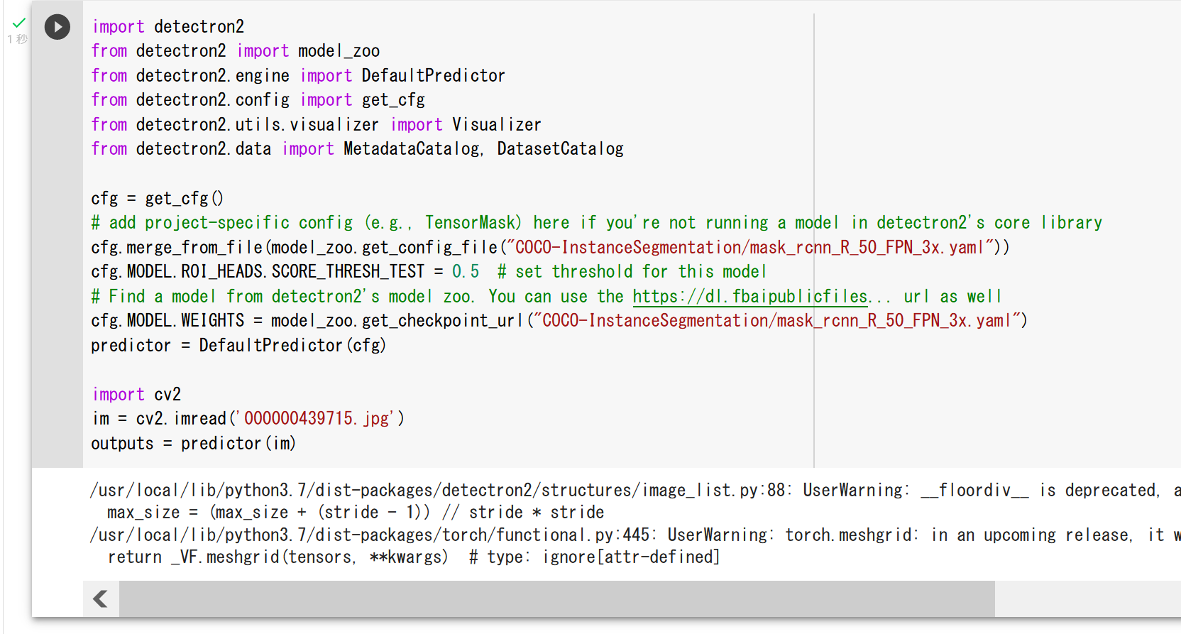
- インスタンス・セグメンテーションの結果の確認
https://colab.research.google.com/drive/16jcaJoc6bCFAQ96jDe2HwtXj7BMD_-m5#scrollTo=FsePPpwZSmqt の記載による.
# look at the outputs. See https://detectron2.readthedocs.io/tutorials/models.html#model-output-format for specification
print(outputs["instances"].pred_classes)
print(outputs["instances"].pred_boxes)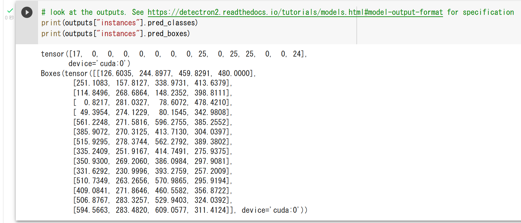
- インスタンス・セグメンテーションの結果の表示
https://colab.research.google.com/drive/16jcaJoc6bCFAQ96jDe2HwtXj7BMD_-m5#scrollTo=FsePPpwZSmqt の記載による.
# We can use `Visualizer` to draw the predictions on the image.
v = Visualizer(im[:, :, ::-1], MetadataCatalog.get(cfg.DATASETS.TRAIN[0]), scale=1.2)
out = v.draw_instance_predictions(outputs["instances"].to("cpu"))
import matplotlib.pyplot as plt
plt.imshow(out.get_image()[:, :, ::-1])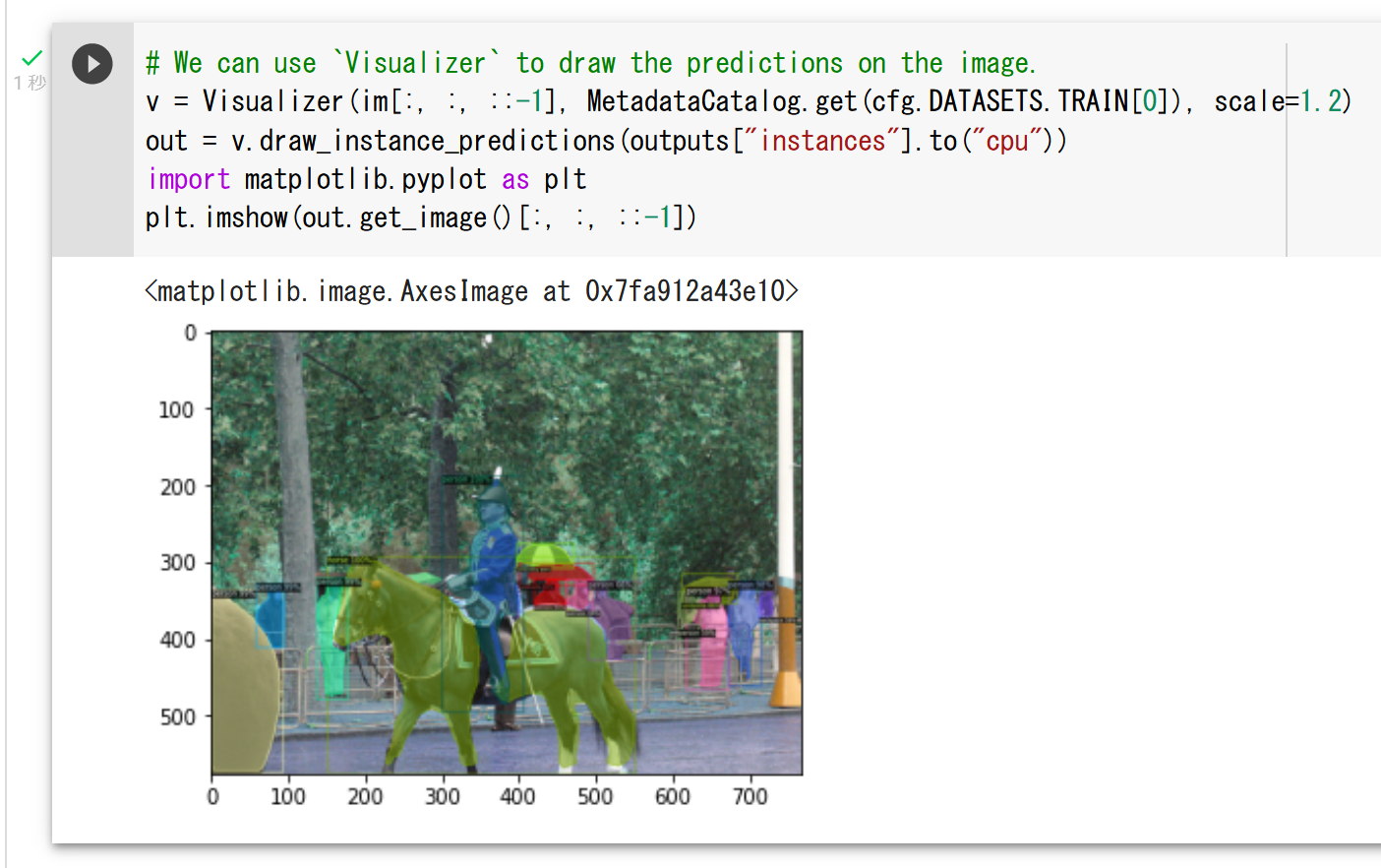
Windows での Detectron2 のインストールと動作確認
別ページ »で説明している.
Linux での Detectron2 のインストール
https://github.com/facebookresearch/detectron2/releases
このページによれば,Linux マシンで,NVIDIA CUDA ツールキット 11.1, PyTorch 1.9 がインストール済みの場合には,次のような手順になる.
python -m pip install detectron2==0.5 -f https://dl.fbaipublicfiles.com/detectron2/wheels/cu111/torch1.9/index.html
DETR
物体検出, panoptic segmentation の一手法.2020年発表.
- 文献
Nicolas Carion, Francisco Massa, Gabriel Synnaeve, Nicolas Usunier, Alexander Kirillov, Sergey Zagoruyko, End-to-End Object Detection with Transformers, ECCV 2020, also CoRR, abs/2005.12872v3, 2020.
- 公式のソースコード (GitHub): https://github.com/facebookresearch/detr
- 公式のデモ (Google Colaboratory): https://colab.research.google.com/github/facebookresearch/detr/blob/colab/notebooks/detr_demo.ipynb
- Papers with Code のページ: https://paperswithcode.com/paper/end-to-end-object-detection-with-transformers
- TensorFlow のモデル: https://github.com/tensorflow/models/tree/master/official/projects/detr
- MMDetection のモデル: https://github.com/open-mmlab/mmdetection/blob/master/configs/detr/README.md
【関連項目】 Deformable DETR, MMDetection, panoptic segmentation, 物体検出
DiffBIR
DiffBIRは画像復元の手法の一つである. 画像復元は,低品質または劣化した画像を元の高品質な状態に修復するタスクである. このタスクでは,ノイズや歪みなどの複雑な問題に対処する必要がある. DiffBIRは,2つの主要なステージから成り立っている. 最初のステージでは,画像復元が行われ,低品質な画像が高品質に修復される. そして,2番目のステージでは,事前に訓練された Stable Diffusion を使用して,高品質な画像が生成される. DiffBIRは他の既存の手法よりも優れた結果を得ることができることが実験によって示されている.
【文献】
Xinqi Lin, Jingwen He, Ziyan Chen, Zhaoyang Lyu, Ben Fei, Bo Dai, Wanli Ouyang, Yu Qiao, Chao Dong, DiffBIR: Towards Blind Image Restoration with Generative Diffusion Prior, arXiv:2308.15070v1, 2023.
https://arxiv.org/pdf/2308.15070v1.pdf
【関連する外部ページ】
- 公式のデモページ(Google Colaboratory 上): https://colab.research.google.com/github/camenduru/DiffBIR-colab/blob/main/DiffBIR_colab.ipynb
- DiffBIR の公式の GitHub のページ: https://github.com/XPixelGroup/DiffBIR
- Papers with Code のページ: https://paperswithcode.com/paper/diffbir-towards-blind-image-restoration-with
diffusion model
Jascha Sohl-Dickstein, Eric A. Weiss, Niru Maheswaranathan, Surya Ganguli, Deep Unsupervised Learning using Nonequilibrium Thermodynamics, arXiv:1503.03585 [cs.LG].
Dlib
Dlib は,数多くの機能を持つソフトウェアである. Python, C++ のプログラムから使うためのインタフェースを持つ.
Dlib の機能には,機械学習,数値計算,グラフィカルモデル推論,画像処理,スレッド,通信,GUI,データ圧縮・一貫性,テスト,さまざまなユーティリティがある.
Dlib には,顔情報処理に関して,次の機能がある.
- 顔検出 (face detection)
- 顔ランドマーク (facial landmark)の検出
- 顔のアラインメント
- 顔のコード化
ディープニューラルネットワークの学習済みモデルも配布されている.
Dlib の URL: http://dlib.net/
【関連項目】 FairFace, Max-Margin 物体検出 , 顔検出 (face detection), 顔ランドマーク (facial landmark), 顔のコード化
Windows での Dlib のインストール
Dlib のインストールは,複数の方法がある.
- Windows での Dlib,face_recognition のインストール(ソースコードを使用): 別ページ »で説明している.
- Windows での Python の Dlib ライブラリのインストール,Dlib のソースコード等と,Dlib の学習済みモデルのダウンロード: 別ページ »で説明している.
私がビルドしたもの,非公式,無保証. 公開されている Dlib のソースコードを改変せずにビルドした. Windows 10, Build Tools for Visual Studio 2022 を用いてビルドした.NVIDIA CUDA は使用せずにビルドした. Eigen の MPL2 ライセンスによる.
zip ファイルは C:\ 直下で展開し,C:\dlib での利用を想定している.
Ubuntu での Dlib のインストール
Dlib の顔検出
Dlib の顔検出 は次の仕組みで行われる.
Dlib には,ディープラーニングの CNN (convolutional neural network) を用いた物体検出 が実装されている. そこでは,Max-Margin 物体検出法が利用されている(文献は次の通り). それにより,Dlib の顔検出 が行われる.
Davis E. King, Max-Margin Object Detection, CoRR, abs/1502.00046, 2015
- 前準備として,パッケージのインストールと,学習済みモデルのダウンロードを行う.
ここでダウンロードしている mmod_human_face_detector.dat は,学習済みモデルのファイルである. ImageNet データセット, AFLW, Pascal VOC, VGG, WIDER FACE データセット, face scrub 画像について, Dlib の作者がアノテーションしたものを用いて学習済みである. 詳細は https://github.com/davisking/dlib-models を参照のこと.
Windows では, コマンドプロンプトを管理者として開き次のコマンドを実行する.
python -m pip install dlib opencv-python matplotlib
curl -O http://dlib.net/files/mmod_human_face_detector.dat.bz2
"c:\Program Files\7-Zip\7z.exe" x mmod_human_face_detector.dat.bz2
Linux では次のコマンドを実行する.
# パッケージリストの情報を更新 sudo apt update sudo apt -y install python3-matplotlib libopencv-dev libopencv-core-dev python3-opencv libopencv-contrib-dev opencv-data sudo pip3 install dlib curl -O http://dlib.net/files/mmod_human_face_detector.dat.bz2 bzip2 -d mmod_human_face_detector.dat.bz2 - Dlib を用いた顔検出の Python プログラムは次の通りである.
import dlib import cv2 %matplotlib inline import matplotlib.pyplot as plt import warnings warnings.filterwarnings('ignore') # Suppress Matplotlib warnings import time import argparse # 使い方: 次のプログラムを a.py というファイル名で保存し,「python a.py」のように実行. # あるいは python a.py --image IMG_3264.png --model mmod_human_face_detector.dat のように. # --model は学習済みモデルのファイル名を指定できる ap = argparse.ArgumentParser() ap.add_argument("-i", "--image", help="input image", default="a.png") ap.add_argument("-m", "--model", help="pre-trained model", default="python_examples/mmod_human_face_detector.dat") ap.add_argument("-u", "--upsample", type=int, default=1) args = vars(ap.parse_args()) # face_detector = dlib.cnn_face_detection_model_v1(args['model']) # 画像ファイル名を a.png のところに設定 bgr = cv2.imread(args['image']) if bgr is None: print("画像ファイルがない") exit() # 顔検出を行う. start = time.time() faces = face_detector(cv2.cvtColor(bgr, cv2.COLOR_BGR2RGB), args['upsample']) end = time.time() print("秒数 : ", format(end - start, '.2f')) # 顔検出で得られた顔(複数あり得る)それぞれについて,赤い四角を書く for i, f in enumerate(faces): x = f.rect.left() y = f.rect.top() width = f.rect.right() - x height = f.rect.bottom() - y cv2.rectangle(bgr, (x, y), (x + width, y + height), (0, 0, 255), 2) print("%s, %d, %d, %d, %d" % (args['image'], x, y, x + width, y + height)) # 画面に描画 plt.style.use('default') plt.imshow(cv2.cvtColor(bgr, cv2.COLOR_BGR2RGB)) # ファイルに保存 cv2.imwrite("result.png", bgr) - 次のような結果が表示される.
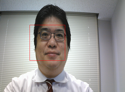
次のページは,上のプログラム等を記載したGoogle Colaboratory のページである.ページを開き実行できる.
URL: https://colab.research.google.com/drive/1q-dGCfre8MT5Zet2O3xYoYMUP0sx_KLc?usp=sharing [Google Colaboratory]
Dlib の顔検出の詳しい手順: 別ページ »で説明している.
DreamGaussian
DreamGaussianは3Dコンテンツ生成のフレームワークであり,画像から3Dモデルを生成する(Image-to-3D)とテキストから3Dモデルを生成する(Text-to-3D)の二つの主要なタスクに対応している.既存の手法である Neural Radiance Fields(NeRF)は高品質な結果を出すものの,計算時間が長いという課題があった.DreamGaussianの特長は,3Dガウススプラッティングモデルを用いることで,メッシュの抽出とUV空間でのテクスチャの精緻化が効率的に行える点である.このアプローチにより,DreamGaussianは既存の NeRF ベースの手法よりも高速な3Dコンテンツ生成を実現している.さらに,実験結果では,DreamGaussianが Image-to-3D と Text-to-3D の両方のタスクで既存の方法よりも高速であることが確認されている.
【文献】
Jiaxiang Tang, Jiawei Ren, Hang Zhou, Ziwei Liu, Gang Zeng, DreamGaussian: Generative Gaussian Splatting for Efficient 3D Content Creation, arXiv:2309.16653v1, 2023.
https://arxiv.org/pdf/2309.16653v1.pdf
【関連する外部ページ】
- 公式のオンラインデモ(Google Colaboratory): https://colab.research.google.com/drive/1sLpYmmLS209-e5eHgcuqdryFRRO6ZhFS?usp=sharing
- Image-to-3D の公式のオンラインデモ(Google Colaboratory): https://colab.research.google.com/drive/1sLpYmmLS209-e5eHgcuqdryFRRO6ZhFS?usp=sharing
元画像

中間結果(左),最終結果のスクリーンショット(右)
処理結果(3次元データ): b.obj, b.mtl, b_albedo.png
処理結果のスクリーンショット(動画):
- Text-to-3D の公式のオンラインデモ(Google Colaboratory): https://colab.research.google.com/github/camenduru/dreamgaussian-colab/blob/main/dreamgaussian_colab.ipynb

処理結果(3次元データ): icecream_mesh.obj, icecream_mesh.mtl, icecream_mesh_albedo.png, icecream_model.ply
処理結果のスクリーンショット(動画): icecream.mp4
- GitHub のページ: https://github.com/dreamgaussian/dreamgaussian
- Papers with Code のページ: https://paperswithcode.com/paper/dreamgaussian-generative-gaussian-splatting
DUTS データセット
DUTS データセットは,saliency detection のためのデータセットである. 10,553枚の訓練画像と5,019枚のテスト画像を含む.
- 訓練画像は ImageNet DET training/val set から収集された.
- テスト画像は ImageNet DET training/val set と SUN データセットから収集された.
いずれも手動でアノテーションされている.
次の URL で公開されているデータセット(オープンデータ)である.
URL: http://saliencydetection.net/duts/
- Papers with Code: https://paperswithcode.com/dataset/duts
- ImageNet データセットの文献
J. Deng, W. Dong, R. Socher, L.-J. Li, K. Li, and L. Fei-Fei, Imagenet: A large-scale hierarchical image database, CVPR, 2009.
- SUN データセットの文献
J. Xiao, J. Hays, K. A. Ehinger, A. Oliva, and A. Torralba, SUN database: Large-scale scene recognition from abbey to zoo, CVPR, 2010.
- DUTS データセットの文献
Lijun Wang, Huchuan Lu, Yifan Wang, Mengyang Feng, Dong Wang, Baocai Yin, and Xiang Ruan, Learning to detect salient objects with image-level supervision, CVPR, 2017.
https://openaccess.thecvf.com/content_cvpr_2017/papers/Wang_Learning_to_Detect_CVPR_2017_paper.pdf
【関連項目】 salient object detection, 物体検出
Early Stopping
Early Stopping は, 正則化 (regularization) のための一手法である. training loss の減少が終わるのを待たずに,学習の繰り返しを打ち切る. このとき,検証用データでの検証において,validation loss が増加を開始した時点で,学習の繰り返しを打ち切る.
【Keras のプログラム】
from keras.callbacks import EarlyStopping
cb = EarlyStopping(monitor='val_loss', patience = 10)
コールバックは,次のようにして使用する.
【Keras のプログラム】
history = m.fit(x_train, y_train, batch_size=32, epochs=50, validation_data=(x_test, y_test), callbacks=[cb])
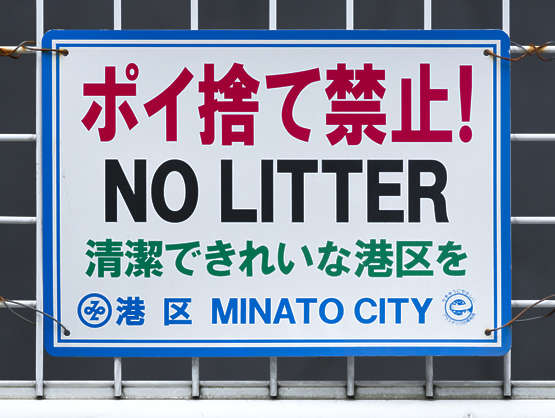
EasyOCR
EasyOCR は,多言語の文字認識のソフトウエアである. テキスト検出に CRAFT を使用している.
学習用のソースコードも公開されている.
【サイト内の関連ページ】
EasyOCR のインストールと動作確認(多言語の文字認識)(Python,PyTorch を使用)(Windows 上): 別ページ »で説明している.
【関連する外部ページ】
- 公式の GitHub のページ: https://github.com/JaidedAI/EasyOCR
- 公式のオンラインデモ: https://www.jaided.ai/easyocr/
【関連項目】 CRAFT, OCR
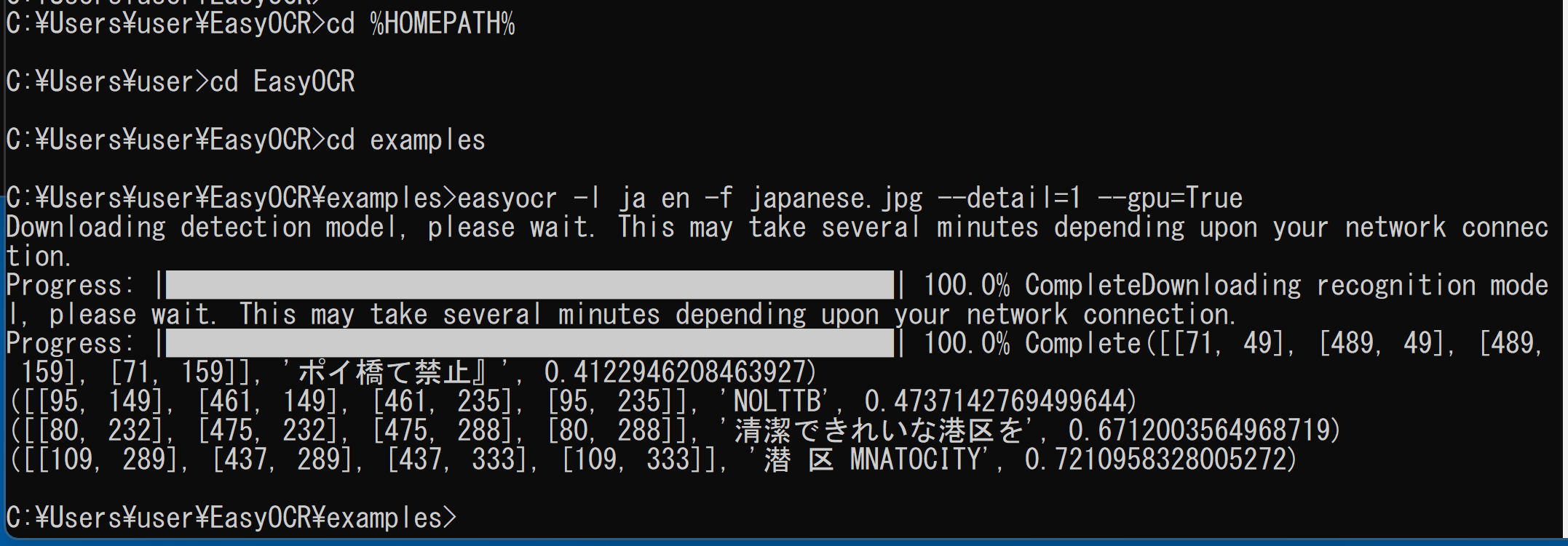
Google Colaboratory で,EasyOCR による日本語読み取りの実行
公式の手順 (https://github.com/JaidedAI/EasyOCR)による.
次のコマンドやプログラムは Google Colaboratory で動く(コードセルを作り,実行する).
- EasyOCR のインストール
!pip3 install git+git://github.com/jaidedai/easyocr.git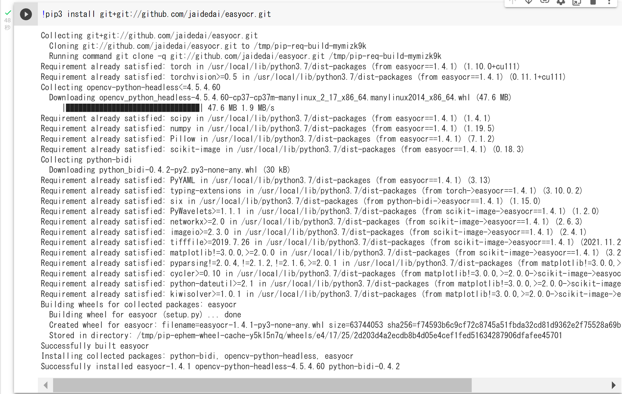
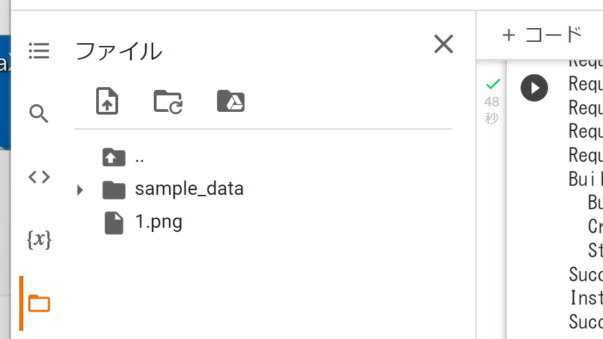
- 処理したい画像ファイルを Google Colaboratory にアップロードする.
- OCR の実行
「ja」は「日本語」の意味である.
import easyocr
reader = easyocr.Reader(['ja'])
result = reader.readtext('1.png')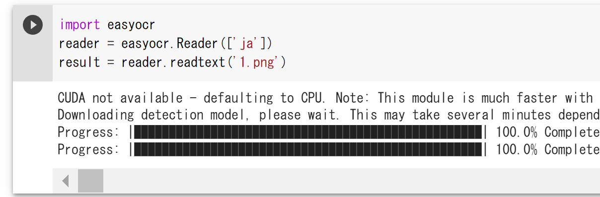
- 結果の確認
from IPython.display import display
display(result)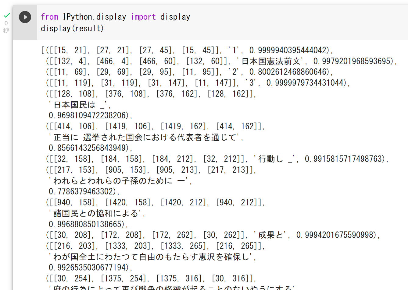
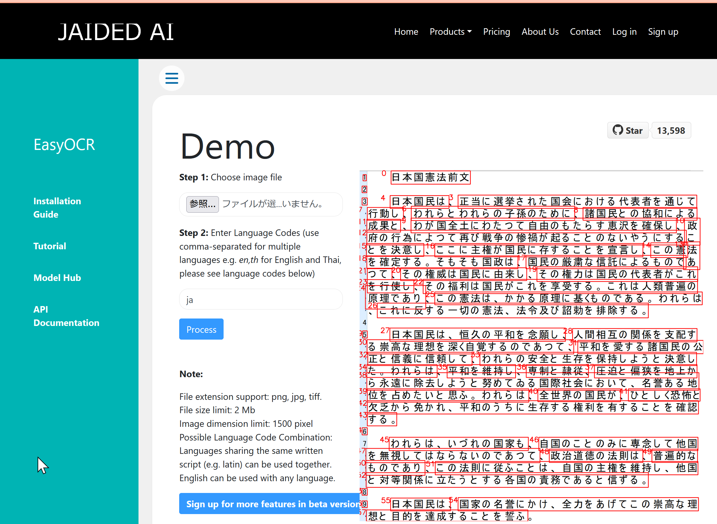
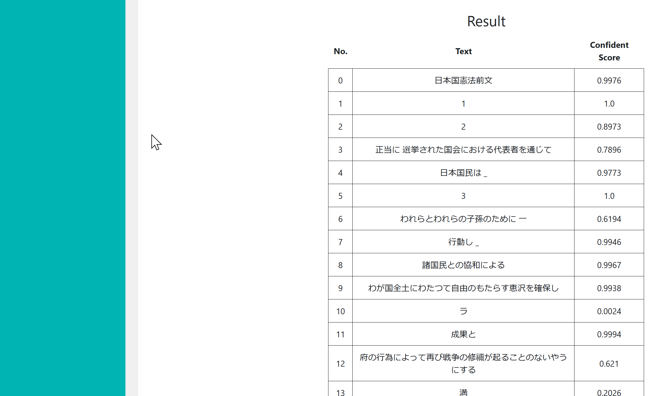
JAIDED AI による EasyOCR のオンラインデモ
JAIDED AI による EasyOCR のオンラインデモの URL: https://www.jaided.ai/easyocr/
EdgeBoxes 法
エッジから,オブジェクトのバウンディングボックス(包含矩形)を求める方法である.
- 文献
C. L. Zitnick and P. Dollár. Edge boxes: Locating object proposals from edges, ECCV, 2014.
- Papers with Code の EdgeBoxes のページ: https://paperswithcode.com/method/edgeboxes
【関連項目】 物体検出
EfficientDet
zylo117 による EfficientDet の実装 (GitHub) のページ: https://github.com/zylo117
【関連項目】 物体検出
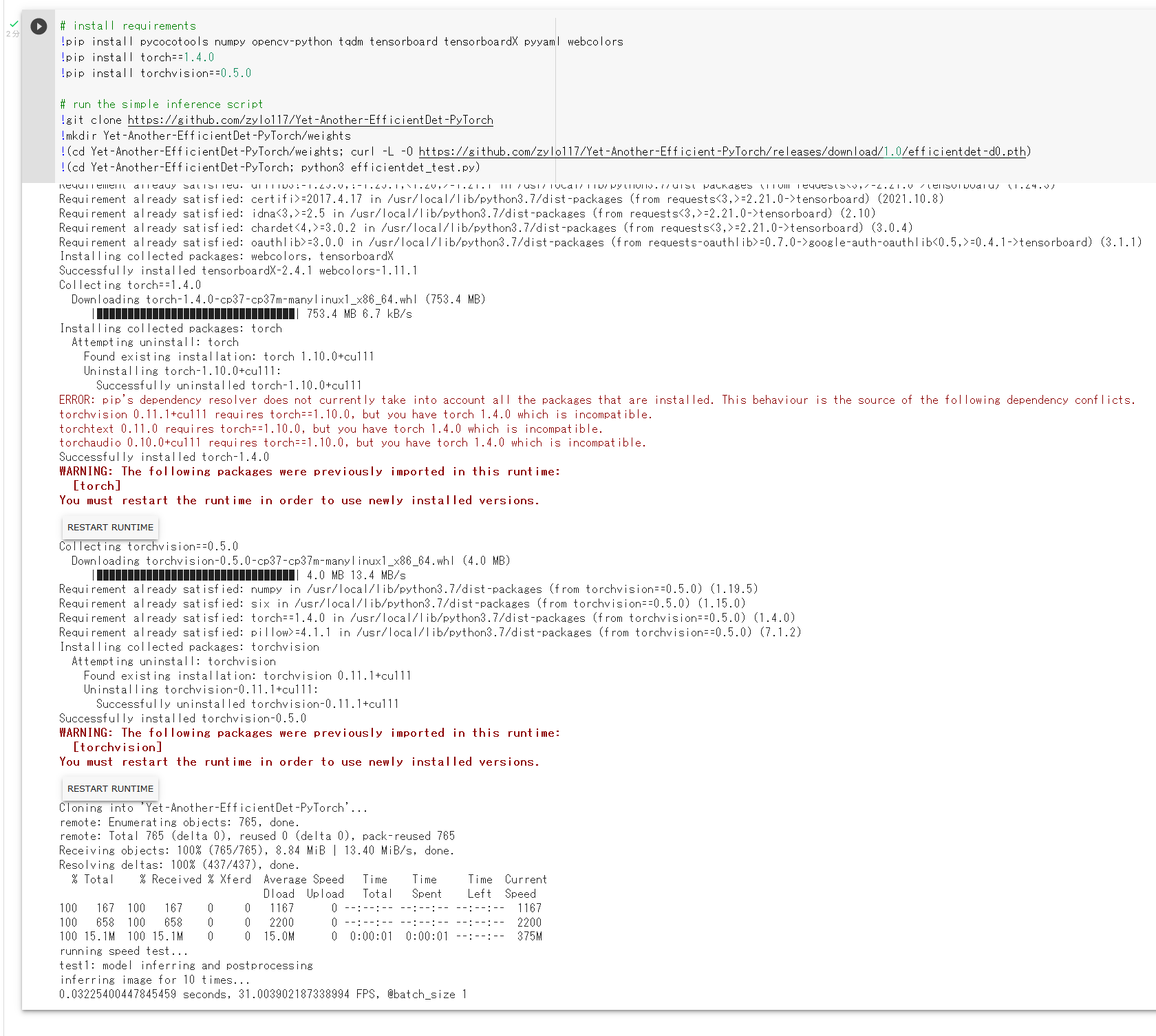
Google Colaboratory で,EfficientDet のインストール
次のコマンドやプログラムは Google Colaboratory で動く(コードセルを作り,実行する).
# install requirements
!pip3 install pycocotools numpy opencv-python opencv-contrib-python tqdm tensorboard tensorboardX pyyaml webcolors
!pip3 install torch==1.4.0
!pip3 install torchvision==0.5.0

# run the simple inference script
!rm -rf Yet-Another-EfficientDet-PyTorch
!git clone https://github.com/zylo117/Yet-Another-EfficientDet-PyTorch
!mkdir Yet-Another-EfficientDet-PyTorch/weights
!(cd Yet-Another-EfficientDet-PyTorch/weights; curl -L -O https://github.com/zylo117/Yet-Another-Efficient-PyTorch/releases/download/1.0/efficientdet-d0.pth)
!(cd Yet-Another-EfficientDet-PyTorch; python3 efficientdet_test.py)
ELSED
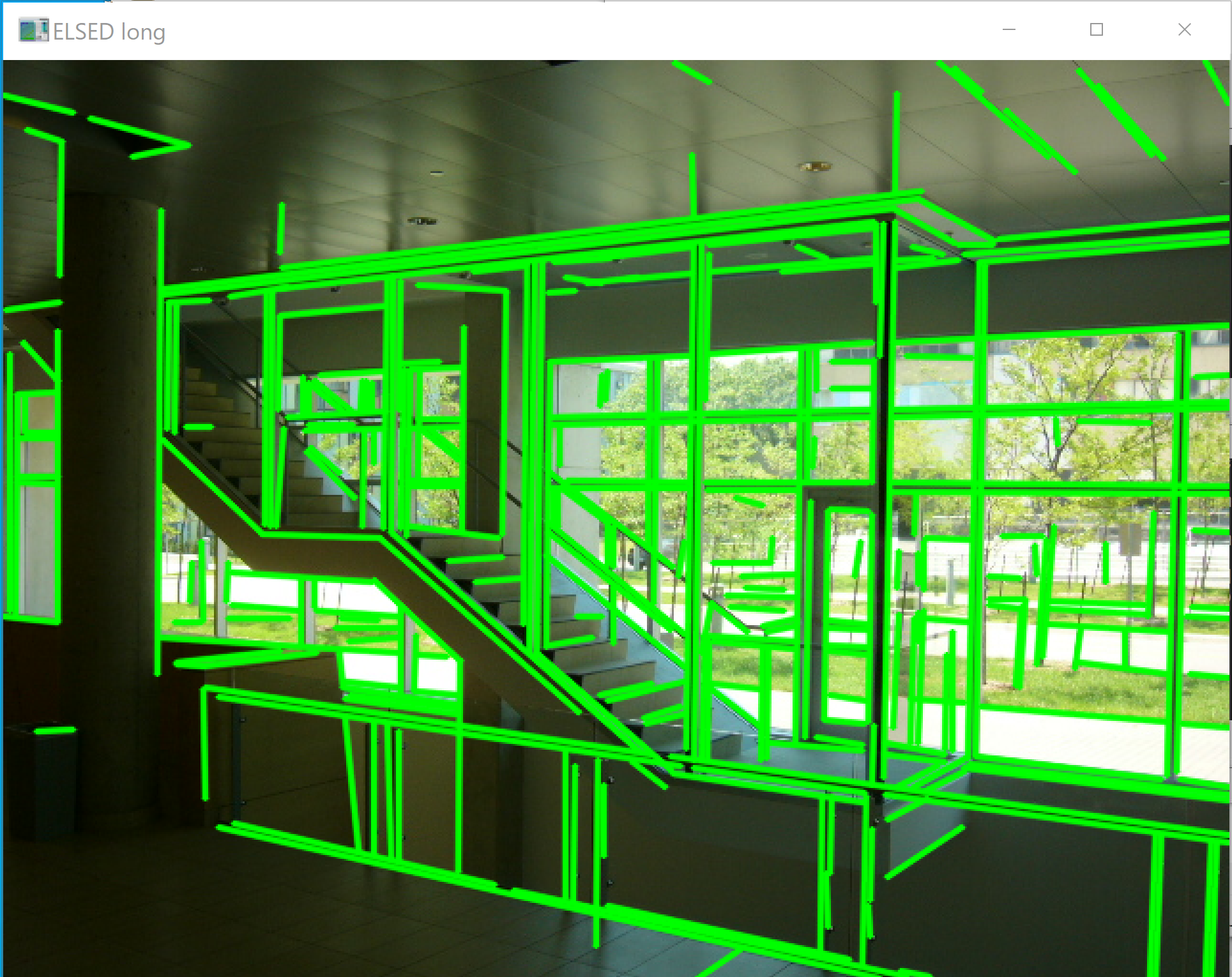
【文献】
Iago Suárez and José M. Buenaposada and Luis Baumela, ELSED: Enhanced Line SEgment Drawing, Pattern Recognition, vol. 127, pages 108619, arXiv:2108.03144, 2022. doi: https://doi.org/10.1016/j.patcog.2022.108619.
arXiv: https://arxiv.org/abs/2108.03144
https://arxiv.org/pdf/2108.03144.pdf
【サイト内の関連ページ】
ELSED のインストールと動作確認(線分検知)(Build Tools, Python を使用)(Windows 上)
【関連する外部ページ】
- ELSED の GitHub のページ: https://github.com/iago-suarez/ELSED
- Google Colab のデモ: https://colab.research.google.com/github/iago-suarez/ELSED/blob/main/Python_ELSED.ipynb
- Papers with Code のページ: https://paperswithcode.com/paper/elsed-enhanced-line-segment-drawing
【関連項目】 線分検知
Emotion-Investigator
SanjayMarreddi の Emotion-Investigator は,顔検出 (face detection)と,Happy, Sad, Disgust, Neutral, Fear, Angry, Surprise の表情推定を行う.
【サイト内の関連ページ】
- 顔検出と表情推定(SanjayMarreddi/Emotion-Investigator,Python,TensorFlow を使用)(Windows 上): 別ページ »で説明している.
【関連する外部ページ】
- SanjayMarreddi/Emotion-Investigator の GitHub の公式ページ: https://github.com/SanjayMarreddi/Emotion-Investigator
ESRGAN
超解像 (super resolution) の一手法.2018 年発表.
- 文献
Wang, Xintao and Yu, Ke and Wu, Shixiang and Gu, Jinjin and Liu, Yihao and Dong, Chao and Qiao, Yu and Loy, Chen Change, ESRGAN: Enhanced super-resolution generative adversarial networks, The European Conference on Computer Vision Workshops (ECCVW), 2018.
- 公式のソースコード: https://github.com/xinntao/ESRGAN
- Papers with Code のページ: https://paperswithcode.com/paper/esrgan-enhanced-super-resolution-generative
- 超解像に関する Google Colaboratory のノートブック: https://colab.research.google.com/github/AwaleSajil/ISR_simplified/blob/master/ISR_simplified(youtube).ipynb#scrollTo=yn2qU_Gstb12
【関連項目】 GAN (Generative Adversarial Network), image super resolution, video super resolution, 超解像 (super resolution)
FaceForensics++ データセット
FaceForensics++ データセットは,自動合成された顔画像のデータセットである.
- FaceForensics++ は,977本の YouTube 動画を使用.Deepfakes, Face2Face, FaceSwap and NeuralTextures を用いて顔データを操作し,1000 個の動画を作成したものである.
- 動画は,オクルージョンのない,ほぼ正面の顔を含むように選択されている.
FaceForensics++ データセットは,次の URL で公開されているデータセット(オープンデータ)である.
URL: https://github.com/ondyari/FaceForensics
【関連情報】
- FaceForensics++: Learning to Detect Manipulated Facial Images, Andreas Rössler, Davide Cozzolino, Luisa Verdoliva, Christian Riess, Justus Thies, Matthias Nießner
- Papers With Code の FaceForensics++ データセットのページ: https://paperswithcode.com/dataset/faceforensics-1
FairFace (Face Attribute Dataset for Balanced Race, Gender, and Age)
性別,年齢,人種に関するバイアス (bias) 等の問題がないとされる顔データセットが発表された.2021年発表. 顔の性別,年齢等の予測の精度向上ができるとされている.
- Karkkainen, Kimmo and Joo, Jungseock, FairFace: Face Attribute Dataset for Balanced Race, Gender, and Age for Bias Measurement and Mitigation, Proceedings of the IEEE/CVF Winter Conference on Applications of Computer Vision, pp. 1548-1558, 2021
- GitHub のページ: https://github.com/dchen236/FairFace
【関連項目】 Dlib, 顔のデータベース, 顔ランドマーク (facial landmark), 顔の性別,年齢等の予測
Google Colaboratory での FairFace デモプログラムの実行
顔の性別,年齢等の予測を行う.
次のコマンドやプログラムは Google Colaboratory で動く(コードセルを作り,実行する).
- Google Colaboratory で,ランタイムのタイプを GPU に設定する.
- ソースコード等のダウンロード
!git clone https://github.com/dchen236/FairFace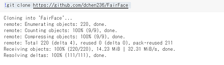
- 公式の GitHub のページの記載により,事前学習済みモデルをダウンロードする.
公式の GitHub のページ: https://github.com/dchen236/FairFace
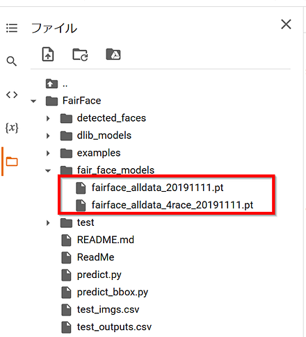
2つのファイルをダウンロードする.
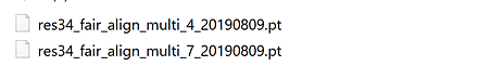
- いまダウンロードしたファイルについて.
Google Colaboratory で「fair_face_models」という名前のディレクトリを作る. そして,いまダウンロードしたファイルのファイル名を次のように変えて, 「fair_face_models」ディレクトリの下に置く. (ファイル名については,predict.py の中で指定されているファイル名にあわせる)
- 実行する.
%cd FairFace
!python3 predict.py --csv test_imgs.csv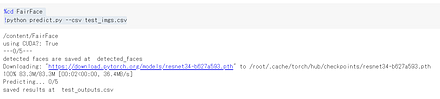
test_imgs.csv には,次の画像ファイルのファイル名が設定されている.
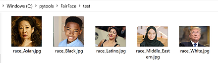 自前の画像で動作確認したいときは,画像ファイル名を書いた csv ファイルを準備する.
 - 実行結果の確認
性別,年齢などが推定されている.
!cat test_outputs.csv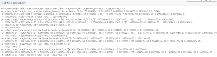
Windows での FairFace デモプログラムの実行
顔の性別,年齢等の予測を行う.
- 前準備として PyTorch, Dlib のインストール,Git のインストール(別項目で説明している)を行っておくこと.
Git の公式ページ: https://git-scm.com/
- ソースコード等のダウンロード
git clone https://github.com/dchen236/FairFace - 公式の GitHub のページの記載により,事前学習済みモデルをダウンロードする.
公式の GitHub のページ: https://github.com/dchen236/FairFace
2つのファイルをダウンロードする.
- いまダウンロードしたファイルについて.
「fair_face_models」という名前のディレクトリを作る. そして,いまダウンロードしたファイルのファイル名を次のように変えて, 「fair_face_models」ディレクトリの下に置く. (ファイル名については,predict.py の中で指定されているファイル名にあわせる)
- 実行する.
cd FairFace
python predict.py --csv test_imgs.csv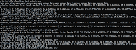
test_imgs.csv には,次の画像ファイルのファイル名が設定されている.
自前の画像で動作確認したいときは,画像ファイル名を書いた csv ファイルを準備する. - 実行結果の確認
性別,年齢などが推定されている.
type test_outputs.csv
Fashion MNIST データセット
Fashion MNIST データセットは,公開されているデータセット(オープンデータ)である.
Fashion MNIST データセットは,10 種類のモノクロ画像と,各画像に付いたラベル(10 種類の中の種類を示す)から構成されるデータセットである.
- 画像の枚数:合計 70000枚.
(内訳)70000枚の内訳は次の通りである.
60000枚:教師データ
10000枚:検証データ
- 画像のサイズ: 28x28 である.
- ラベル
- 0: T-shirt/top
- 1: Trouser
- 2: Pullover
- 3: Dress
- 4: Coat
- 5: Sandal
- 6: Shirt
- 7: Sneaker
- 8: Bag
- 9: Ankle boot
- 画素はグレースケールであり,画素値は0~255である.0が白,255が黒.
【文献】
Han Xiao, Kashif Rasul, and Roland Vollgraf, Fashion-MNIST: a Novel Image Dataset for Benchmarking Machine Learning Algorithms, arXiv:1708.07747 [cs.LG], 2017.
【サイト内の関連ページ】
- Fashion MNIST データセットを扱う Python プログラム: 別ページ で説明している.
- Fashion MNIST データセットによる学習と分類(TensorFlow データセット,TensorFlow,Python を使用)(Windows 上,Google Colaboratory の両方を記載)
【関連する外部ページ】
- 公式ページ: https://github.com/zalandoresearch/fashion-mnist
- TensorFlow データセットの Fashion MNIST データセット: https://www.tensorflow.org/datasets/catalog/fashion_mnist
【関連項目】 Keras に付属のデータセット, MNIST データセット, TensorFlow データセット, オープンデータ, 画像分類
Python での Fashion MNIST データセットのロード(TensorFlow データセットを使用)
次の Python プログラムは,TensorFlow データセットから,Fashion MNIST データセットのロードを行う. x_train, y_train が学習用のデータ,x_test, y_test が検証用のデータになる.
- x_train: サイズ 28 × 28 の 60000枚の濃淡画像
- y_train: 60000枚の濃淡画像それぞれの,種類番号(0 から 9 のどれか)
- x_test: サイズ 28 × 28 の 10000枚の濃淡画像
- y_test: 10000枚の濃淡画像それぞれの,種類番号(0 から 9 のどれか)
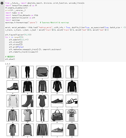
次の Python プログラムでは,TensorFlow データセットから,Fashion MNIST データセットのロードを行う. x_train と y_train を 25枚分表示することにより,x_train と y_train が,モノクロ画像であることが確認できる.
tensorflow_datasets の loadで, 「batch_size = -1」を指定して,一括読み込みを行っている.
from __future__ import absolute_import, division, print_function, unicode_literals
import tensorflow as tf
import numpy as np
import tensorflow_datasets as tfds

%matplotlib inline
import matplotlib.pyplot as plt
import warnings
warnings.filterwarnings('ignore')   # Suppress Matplotlib warnings

# Fashion MNIST データセットのロード
fashion_mnist, fashion_mnist_metadata = tfds.load('fashion_mnist', with_info = True, shuffle_files=True, as_supervised=True, batch_size = -1)
x_train, y_train, x_test, y_test = fashion_mnist['train'][0], fashion_mnist['train'][1], fashion_mnist['test'][0], fashion_mnist['test'][1]

plt.style.use('default')
plt.figure(figsize=(10,10))
for i in range(25):
    plt.subplot(5,5,i+1)
    plt.xticks([])
    plt.yticks([])
    plt.grid(False)
# squeeze は,サイズ1の次元を削除.numpy は tf.Tensor を numpy に変換
    plt.imshow(np.squeeze(x_train[i]), cmap=plt.cm.binary)
    plt.xlabel(y_train[i].numpy())

# 確認表示
plt.show()
Python での Fashion MNIST データセットのロード(Keras を使用)
次の Python プログラムは,Keras に付属のデータセットの中にある Fashion MNIST データセットのロードを行う. x_train, y_train が学習用のデータ,x_test, y_test が検証用のデータになる.
- x_train: サイズ 28 × 28 の 60000枚の濃淡画像
- y_train: 60000枚の濃淡画像それぞれの,種類番号(0 から 9 のどれか)
- x_test: サイズ 28 × 28 の 10000枚の濃淡画像
- y_test: 10000枚の濃淡画像それぞれの,種類番号(0 から 9 のどれか)
from tensorflow.keras.datasets import fashion_mnist
(x_train, y_train), (x_test, y_test) = fashion_mnist.load_data()
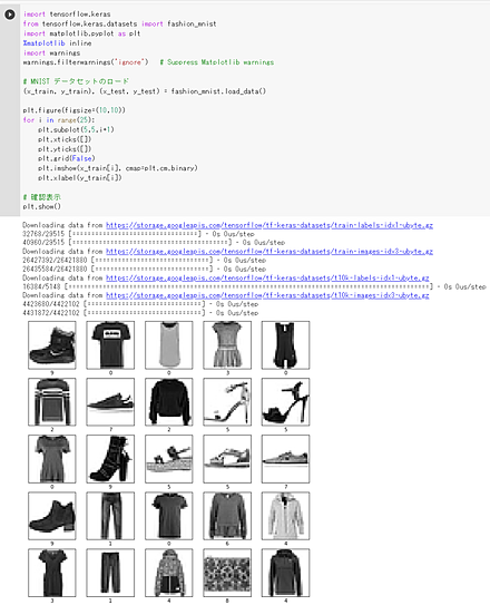
次の Python プログラムは,Keras に付属のデータセットの中にある Fashion MNIST データセットのロードを行う. x_train と y_train を 25枚分表示することにより,x_train と y_train が,モノクロ画像であることが確認できる.
import tensorflow.keras
from tensorflow.keras.datasets import fashion_mnist
%matplotlib inline
import matplotlib.pyplot as plt
import warnings
warnings.filterwarnings('ignore')   # Suppress Matplotlib warnings

# Fashion MNIST データセットのロード
(x_train, y_train), (x_test, y_test) = fashion_mnist.load_data()

plt.style.use('default')
plt.figure(figsize=(10,10))
for i in range(25):
    plt.subplot(5,5,i+1)
    plt.xticks([])
    plt.yticks([])
    plt.grid(False)
    plt.imshow(x_train[i], cmap=plt.cm.binary)
    plt.xlabel(y_train[i])

# 確認表示
plt.show()
TensorFlow データセットからのロード,学習のための前処理
【TensorFlow データセット から Fashion MNIST データセット をロード】
- x_train: サイズ 28 × 28 の 60000枚の濃淡画像
- y_train: 60000枚の濃淡画像それぞれの,種類番号(0 から 9 のどれか)
- x_test: サイズ 28 × 28 の 10000枚の濃淡画像
- y_test: 10000枚の濃淡画像それぞれの,種類番号(0 から 9 のどれか)
結果は,TensorFlow の Tensor である.
type は型,shape はサイズ,np.max と np.min は最大値と最小値である.
tensorflow_datasets の loadで, 「batch_size = -1」を指定して,一括読み込みを行っている.
from __future__ import absolute_import, division, print_function, unicode_literals
import tensorflow as tf
import numpy as np
import tensorflow_datasets as tfds

%matplotlib inline
import matplotlib.pyplot as plt
import warnings
warnings.filterwarnings('ignore')   # Suppress Matplotlib warnings

# Fashion MNIST データセットのロード
fashion_mnist, fashion_mnist_metadata = tfds.load('fashion_mnist', with_info = True, shuffle_files=True, as_supervised=True, batch_size = -1)
x_train, y_train, x_test, y_test = fashion_mnist['train'][0], fashion_mnist['train'][1], fashion_mnist['test'][0], fashion_mnist['test'][1]
print(fashion_mnist_metadata)
# 【x_train, x_test, y_train, y_test の numpy ndarray への変換と,値の範囲の調整(値の範囲が 0 〜 255 であるのを,0 〜 1 に調整)】
x_train = x_train.numpy().astype("float32") / 255.0
x_test = x_test.numpy().astype("float32") / 255.0
y_train = y_train.numpy()
y_test = y_test.numpy()
print(type(x_train), x_train.shape, np.max(x_train), np.min(x_train))
print(type(x_test), x_test.shape, np.max(x_test), np.min(x_test))
print(type(y_train), y_train.shape, np.max(y_train), np.min(y_train))
print(type(y_test), y_test.shape, np.max(y_test), np.min(y_test))
Fast-Robust-ICP
ICP の一手法である.
Fast-Robust-ICP のページ(GitHub): https://github.com/yaoyx689/Fast-Robust-ICP
【関連項目】 K 近傍探索 (K nearest neighbour), ICP
Google Colaboratory で,Fast-Robust-ICP の実行
次のコマンドやプログラムは Google Colaboratory で動く(コードセルを作り,実行する).
- インストール
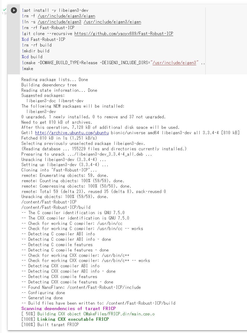
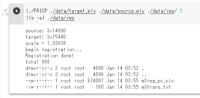
- Fast-Robust-ICP の実行
実行でのオプションについては,Fast-Robust-ICP のページ(GitHub): https://github.com/yaoyx689/Fast-Robust-ICP を参照のこと.
Windows での Fast-Robust-ICP のインストール
ソースコードからビルドする.
- Windows では,前準備として次を行う.
- Build Tools for Visual Studio 2022 のインストール(別項目で説明している).
- Git のインストール(別項目で説明している).
Git の公式ページ: https://git-scm.com/
- cmake のインストール(別項目で説明している).
CMake の公式ダウンロードページ: https://cmake.org/download/
- Eigen 3 のインストール
-
コマンドプロンプトを管理者として開き次のコマンドを実行する.
c:\Fast-Robust-ICP にインストールされる.
cd /d c:%HOMEPATH%
rmdir /s /q Fast-Robust-ICP
git clone --recursive https://github.com/yaoyx689/Fast-Robust-ICP
cd Fast-Robust-ICP
rmdir /s /q build
mkdir build
cd build
del CMakeCache.txt
rmdir /s /q CMakeFiles
cmake -A x64 -T host=x64 ^
    -DCMAKE_INSTALL_PREFIX="c:/Fast-Robust-ICP" ^
    -DEIGEN3_INCLUDE_DIRS="c:/eigen/include;c:/eigen/include/eigen3" ^
..
mklink c:\eigen\include\eigen c:\eigen\include\eigen3
cmake --build . --config Release
del c:\eigen\include\eigen
FERET データベース
FERET データベースは顔のデータベースである.詳細情報は,次の Web ページにある.
https://www.nist.gov/itl/products-and-services/color-feret-database
【関連項目】 顔のデータベース
FFHQ (Flickr-Faces-HQ) データセット
FFHQ (Flickr-Faces-HQ) データセット は,70,000枚の顔画像データセットである. 機械学習による顔の生成などの学習や検証に利用できるデータセットである.
- サイズ 1024×1024,70,000枚の画像
- 年齢,民族,画像背景はさまざま
- 眼鏡,サングラス,帽子などもさまざま
- Flickr から取得.位置合わせとトリミング済み(Dlib を使用),画像の選別, 顔の彫刻や顔の絵画や顔の写真を除去(Amazon Mechanical Turk を使用)
FFHQ (Flickr-Faces-HQ) データセットは次の URL で公開されているデータセット(オープンデータ)である.
URL: https://github.com/NVlabs/ffhq-dataset
【関連情報】
- 文献
A Style-Based Generator Architecture for Generative Adversarial Networks, Tero Karras (NVIDIA), Samuli Laine (NVIDIA), Timo Aila (NVIDIA), CoRR, abs/1812.04948
- Papers With Code の FFHQ データセットのページ: https://paperswithcode.com/dataset/ffhq
【関連項目】 顔のデータベース
FIDTM (FIDT map)
FIDTM (Focal Inverse Distance Transform Map) は, crowd counting の一手法である.2021年発表.
従来の density maps での課題を解決し,従来法よりも精度が上回るとされる. FIDT map を用いて頭部を得る LMDS もあわせて提案されている.
- 文献
Focal Inverse Distance Transform Maps for Crowd Localization and Counting in Dense Crowd, Liang, Dingkang and Xu, Wei and Zhu, Yingying and Zhou, Yu, arXiv preprint arXiv:2102.07925, 2021.
- FIDTM の公式のソースコード
- NWPU-Crowd データセットのダウンロード URL: https://drive.google.com/file/d/1drjYZW7hp6bQI39u7ffPYwt4Kno9cLu8/view
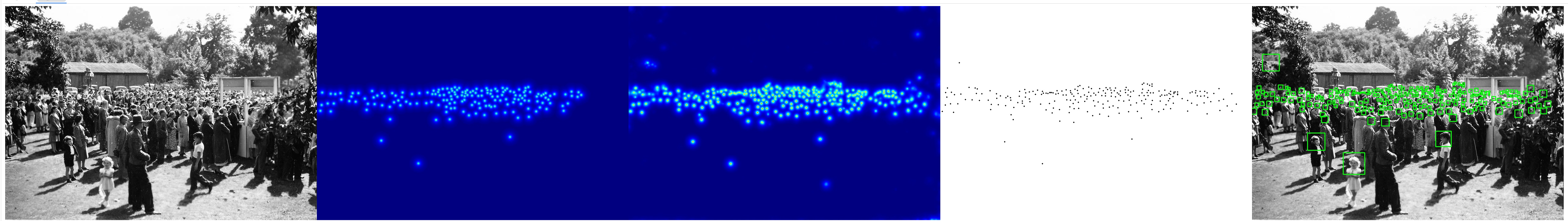
crowd counting の結果の例
- Google Colaboratory のページ
群衆の数のカウントと位置の把握 (crowd counting) (FIDTM を使用)
このページでは,FIDTMの作者による公式のプログラムおよび学習済みモデルを使用して,群衆の数のカウントと位置の把握 (crowd counting) を行う手順を示している.
手順は,FIDTM 公式ページの説明通りに進める.このページでは,Google Colaboratory で簡単に実行できるように,いくつかのコマンドを補っている.説明も補っている.
【関連項目】 crowd counting, JHU-CROWD++ データセット, NWPU-Crowd データセット, ShanghaiTech データセット, UCF-QNRF データセット
fine tuning (ファイン・チューニング)
学習済みモデルを使用する. 学習済みモデルの一部に新しいモデルを合わせた上で,追加のデータを使い学習を行う. このとき,学習済みモデルの部分と,新しいモデルの部分の両方について,パラメータ(重みなど)の調整を行う.
【関連項目】 画像分類 (image classification), 分類, 物体検出
画像分類のモデル DETR でのファイン・チューニング(woctezuma の Google Colaboratory のページを使用)
woctezuma の Google Colaboratory のページを使用する.
このプログラムは,物体検出等の機能を持つモデルである DETR を使い, fine tuning (ファイン・チューニング)と,物体検出を行う.
COCO データセットで学習済みの DETR について,確認のため, 物体検出を行ったあと, 風船(balloon)についてのfine tuning (ファイン・チューニング)を行い, 風船(balloon)が検出できるようにしている. 風船(balloon)は,COCO データセット には無い.
- woctezuma の Google Colaboratory のページを開く.
- torch 1.8.0, torchvision 0.9.0, torchtext 0.9.0 を使うように書き換える.
!pip3 uninstall -y torchtext
!pip3 install torch==1.8.0 torchvision==0.9.0 torchtext==0.9.0
import torch, torchvision
print(torch.__version__, torch.cuda.is_available())

torch.set_grad_enabled(False);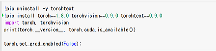
- ソースコードの要点を確認する.
COCO データセットのクラス名を確認する.
orange, apple, banana, dog, person などがある.balloon は無い.
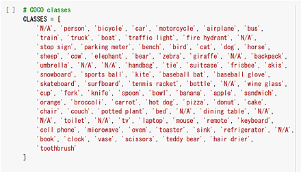
detr_resnet50 の事前学習済みのモデルをダウンロードしている.

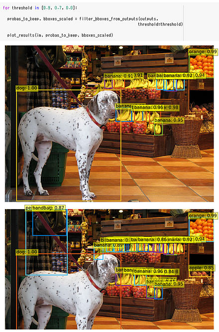
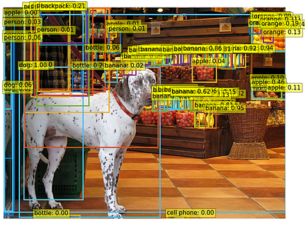
しきい値 0.9, 0.7, 0.0 の 3 通りで実行.しきい値を下げるほど,検出できる物体は増えるが,誤検知も増える傾向にある.
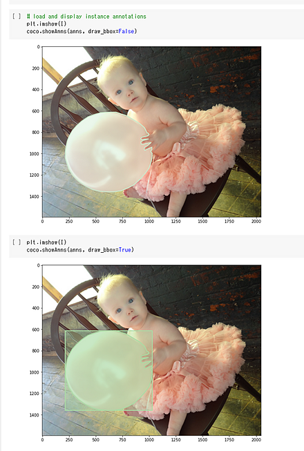
fine tuning を行うため,風船 (balloon) の画像,そして,風船の領域を示した情報(輪郭線,包含矩形)の情報を使う. 画像は複数.そのうち1枚は次の通りである.
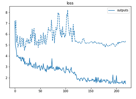
過学習は起きていないようである.
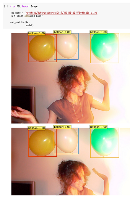
fine tuning により,風船(balloon)を検出できるようになった. しきい値は 0.9, 0.7 の 2通りである.
- 自前のデータで fine tuning を行いたいときは,このページの説明通り,COCO データのフォーマットでデータを準備する.
そのフォーマットは,/content/data/custom (Google Colaboratory の data/custom の下のファイル)が参考になる.
自前のデータが準備できたら,Google Colaboratory にアップロードし, 次のコードセルの「/content/data/custom」のところを書き換えて,再度実行する.
画像ファイルをアップロードし,プログラムは次のように書き換える.
fname = '/content/5m126sn2pov30qzu3pc49lampcp6.jpg'
im = Image.open(fname)
scores, boxes = detect(im, detr, transform)
URL: https://github.com/woctezuma/finetune-detr
FlexGen
FlexGen は,大規模言語モデル (large language model) を用いた推論で必要とされる計算とメモリの要求を削減する技術である. 実験では,大規模言語モデル OPT を,16GB の単一 GPU で実行したとき 100倍以上の高速化が可能であるとされている.
【文献】
Ying Sheng, Lianmin Zheng, Binhang Yuan, Zhuohan Li, Max Ryabinin, Beidi Chen, Percy Liang, Ce Zhang, Ion Stoica, Christopher Ré, High-throughput Generative Inference of Large Language Model with a Single GPU, 2023.
【サイト内の関連ページ】
- FlexGen のインストールと動作確認(大規模言語モデル,チャットボット)(Python,PyTorch を使用)(Windows 上): 別ページ »で説明している.
- Meta の言語モデルと日本語で対話できる chatBOT プログラム(chatBOT)(FlexGen, DeepL, Python を使用)(Windows 上): 別ページ »で説明している.
- 対話システム,chatBOT: PDFファイル, パワーポイントファイル
【関連する外部ページ】
FlexGen の GitHub のページ: https://github.com/FMInference/FlexGen
【関連項目】 OPT
FLIC (Frames Labeled In Cinema)データセット
FLIC は, 5003枚の画像(訓練データ: 3987枚,検証データ: 1016枚)で構成されている. 画像の上半身についてアノテーションが行われている. ほとんどの人物がカメラ正面を向いている.
ディープラーニングにより姿勢推定を行うためのデータとして利用できる.
次の URL で公開されているデータセット(オープンデータ)である.
http://bensapp.github.io/flic-dataset.html
【関連情報】
- 文献
Sapp, B., Taskar, B.: Modec: Multimodal decomposable models for human pose estimation. In: Computer Vision and Pattern Recognition (CVPR), 2013 IEEE Conference on, IEEE (2013) 3674-3681, https://www.cv-foundation.org/openaccess/content_cvpr_2013/papers/Sapp_MODEC_Multimodal_Decomposable_2013_CVPR_paper.pdf
- Papers With Code の FLIC データセットのページ: https://paperswithcode.com/dataset/flic
- TensorFlow データセットの FLIC データセット: https://www.tensorflow.org/datasets/catalog/flic
FordA データセット
FordA データセットは,時系列データである.
FordA データセットは,公開されているデータセット(オープンデータ)である.
URL: http://www.timeseriesclassification.com/description.php?Dataset=FordA
教師データ数:3601
テストデータ数: 1320
モーターセンサーにより計測されたエンジンノイズの計測値である.
FSDnoisy18k データセット
20種類, 約 42.5 時間分のサウンドである.
次の URL で公開されているデータセット(オープンデータ)である.
http://www.eduardofonseca.net/FSDnoisy18k/
- 文献
Eduardo Fonseca, Manoj Plakal, Daniel P. W. Ellis, Frederic Font, Xavier Favory, and Xavier Serra, "Learning Sound Event Classifiers from Web Audio with Noisy Labels", arXiv preprint arXiv:1901.01189, 2019
【関連項目】 sound data
F 検定 (F test)
帰無仮説: 正規分布に従う2群の標準偏差が等しい. F 検定を,t 検定を行う前の等分散性の検定に使うのは正しくないという指摘もある.
var.test(s1, s2)
【関連項目】 検定
GAN (generative adversarial network)
GAN (Generative Adversarial Network) では, 生成器 (generator) でデータを生成し, 識別器 (discriminator) で,生成されたデータが正当か正当でないかを識別する.
- 文献
Ian J. Goodfellow, Jean Pouget-Abadie, Mehdi Mirza, Bing Xu, David Warde-Farley, Sherjil Ozair, Aaron Courville, Yoshua Bengio, Generative Adversarial Networks, Proceedings of the 27th International Conference on Neural Information Processing Systems 2014
- PyTorch-GAN のページ: https://github.com/eriklindernoren/PyTorch-GAN
- Keras-GAN のページ: https://github.com/eriklindernoren/Keras-GAN
- labmlai/annotated_deep_learning_paper_implementations のページ: https://github.com/labmlai/annotated_deep_learning_paper_implementations
【関連項目】 Applications of Deep Neural Networks, Real-ESRGAN, TecoGAN, Wasserstein GAN (WGAN), Wasserstein GAN with Gradient Penalty (WGAN-GP), ディープラーニング
GlueStick
GlueStick 法はイメージ・マッチングの一手法である.2023年発表. 線分を使ったイメージ・マッチングは,照明条件や視点の変化,テクスチャのない領域でもマッチングできるメリットがある. GlueStick 法は,点と線分の両方を利用してイメージ・マッチングを行う. その際に CNN を利用している.
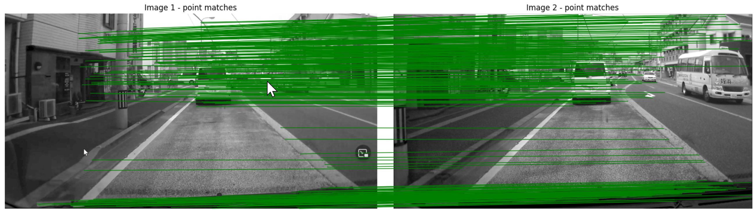
【文献】
Rémi Pautrat, Iago Suárez, Yifan Yu, Marc Pollefeys, Viktor Larsson, GlueStick: Robust Image Matching by Sticking Points and Lines Together, ArXiv, 2023.
https://arxiv.org/pdf/2304.02008v1.pdf
【関連する外部ページ】
- GlueStick の GitHub のページ: https://github.com/cvg/GlueStick
- Google Colab のデモ: https://colab.research.google.com/github/cvg/GlueStick/blob/main/gluestick_matching_demo.ipynb
- Papers with Code のページ: https://paperswithcode.com/paper/gluestick-robust-image-matching-by-sticking
GNN (グラフニューラルネットワーク)
GNN は,グラフ構造を持つデータを用いた学習を可能とする技術である.
【関連項目】 PyTorch Geometric Temporal
He の初期値
He らの方法 (2015年) では,前層のユニット数(ニューロン数)を n とするとき, sqrt( 2 / n ) を標準偏差とする正規分布に初期化する. ただし,この方法は ReLU に特化した手法であるとされている. この方法を使うとき,層の入力は,正規化済みであること.
Kaiming He, Xiangyu Zhang, Shaoqing Ren and Jian Sun, Delving Deep into Rectifiers: Surpassing Human-Level Performance on ImageNet Classification, pp. 1026-1034.
HELEN データセット
HELENデータセットは,顔画像と,顔のパーツの輪郭のデータセットである.
- 400×400 画素の顔画像2330枚
- 目,眉,鼻,唇,顎の輪郭を手動で作成.輪郭は,194個の顔ランドマークで扱う.
次の URL で公開されているデータセット(オープンデータ)である.
http://www.ifp.illinois.edu/~vuongle2/helen/
【関連情報】
- Le V., Brandt J., Lin Z., Bourdev L., Huang T.S. (2012) Interactive Facial Feature Localization. In: Fitzgibbon A., Lazebnik S., Perona P., Sato Y., Schmid C. (eds) Computer Vision - ECCV 2012. ECCV 2012. Lecture Notes in Computer Science, vol 7574. Springer, Berlin, Heidelberg. https://doi.org/10.1007/978-3-642-33712-3_49
- Papers With Code の Helen データセットのページ: https://paperswithcode.com/dataset/helen
【関連項目】 顔のデータベース
HierText データセット
HierTextは,文字認識,レイアウト解析,テキスト検出に利用できるデータセットである.このデータセットには,Open Images データセットから選ばれた11639枚の画像が含まれており,これらの画像はテキストコンテンツとレイアウト構造が豊富である.さらに,約120万語の単語が提供されている.HierText のアノテーションは,単語,行,段落のレベルを含んでいる.訓練セットには8,281枚の画像が含まれ,検証セットには1,724枚の画像が含まれ,さらにテストセットには1,634枚の画像が含まれている.
【サイト内の関連ページ】
HierText データセットのインストール(テキスト検出,文字認識のデータセット)(Windows 上)
【関連する外部ページ】
公式の GitHub のページ: https://github.com/google-research-datasets/hiertext
【関連項目】 Unified Scene Text Detection
HMDB51 (a large human motion database) データセット
HMDB51 (a large human motion database) データセット は,人間の行動データセットである. 機械学習による行動分類,行動認識,ビデオ検索などの学習や検証に利用できるデータセットである.
- 主に映画から収集.その他,Prelinger archive,YouTube,Google video からも収集.
- 6849個のクリップ
- クリップは,アクションカテゴリ(「ジャンプ」,「キス」,「笑い」など)に分類済みである.アクションカテゴリは 51種類.各アクションカテゴリは,最低でも 101個のクリップを含む.
- アクションカテゴリは,次の5つのタイプに分類されている.
HMDB51 (a large human motion database) データセットは次の URL で公開されているデータセット(オープンデータ)である.
https://serre-lab.clps.brown.edu/resource/hmdb-a-large-human-motion-database/#introduction
【関連情報】
- H. Kuehne, H. Jhuang, E. Garrote, T. Poggio and T. Serre, "HMDB: A large video database for human motion recognition," 2011 International Conference on Computer Vision, 2011, pp. 2556-2563, doi: 10.1109/ICCV.2011.6126543.
- Papers With Code の HMDB51 データセットのページ: https://paperswithcode.com/dataset/hmdb51
- PyTorch の HMDB51 データセット: https://pytorch.org/vision/stable/datasets.html#torchvision.datasets.HMDB51
Hourglass Network
Hourglass Network は,stacked hourglass と呼ばれるアーキテクチャを特色とする CNN (convolutional neural network) である.
姿勢推定 (pose estimation) は,画像から,関節 (joint) の (x,y) 座標を得たり, ヒートマップを得る(ヒートマップでは,画素ごとに値を持ち,その値は,関節である確率が高いほど,高い値になる)タスクである. 姿勢推定では,さまざまなスケールでの情報を扱うことが課題とされ, stacked hourglass で解決できるとされている. hourglass では,最初にプーリングを行い,その後アップサンプリングを行う. hourglass を直列に並べて stacked hourglass を構成する.
Hourglass Network の文献は次の通りである.
A. Newell, K. Yang, and J. Deng. Stacked hourglass networks for human pose estimation. In ECCV, 2016, CoRR, abs/1603.06937.
https://arxiv.org/pdf/1603.06937v2.pdf
【関連項目】 姿勢推定
Windows でのインストールと学習
Hourglass Network を用いた姿勢推定については,次の文献がある.
https://github.com/bearpaw/pytorch-pose
上の文献では,ディープラーニングにより,人体全身の姿勢推定を行っている. その学習は,次の手順で行う.
- MPII Human Pose データセット のダウンロードは, https://github.com/bearpaw/pytorch-pose の記載通りに,前もって行っておくこと.
- Git のインストール(別項目で説明している).
Git の公式ページ: https://git-scm.com/
- Python 3.6, Scipy 1.1.0, PyTorch で動く.
git clone https://github.com/bearpaw/pytorch-pose
py -3.6 -m pip install scipy==1.1.0 imutils easydict progress
py -3.6 -m pip install -U torch torchvision torchaudio --extra-index-url https://download.pytorch.org/whl/cu117
cd pytorch-pose
mkdir .\checkpoint
mkdir .\checkpoint\mpii
mkdir .\checkpoint\mpii\hg_s1_b1
# MPII データセットを用いた学習
py -3.6 .\example\main.py --dataset mpii --arch hg --stack 1 --block 1 --features 256 --checkpoint .\checkpoint\mpii\hg_s1_b1 --anno-path .\data\mpii\mpii_annotations.json --image-path .\mpii\images
HQ-SAM (Segment Anything in High Quality)
HQ-SAMは,既存の SAM(Segment Anything Model)を拡張し,より高精度なゼロショットセグメンテーションを実現する手法である.SAM は,プロンプト(点,バウンディングボックス,粗いマスクなど)を入力として,多様なオブジェクトや視覚構造のセグメンテーションを可能にするモデルである.しかし,SAM は細かい構造を持つオブジェクトに対するセグメンテーションが不十分で,その精度に限界がある.この問題を解決するために,HQ-SAMは SAM を拡張している.HQ-SAMでは,SAM のマスクデコーダに新しい学習可能な「HQ-Output Token」を導入している.さらに,グローバルなセマンティックコンテキストとローカルな境界(バウンダリ)の詳細を両方考慮する「Global-local Feature Fusion」も導入されている.複数のデータセットでの実験により,HQ-SAMが高精度なセグメンテーションマスクを生成できることが確認されている.
【文献】
Ke, Lei and Ye, Mingqiao and Danelljan, Martin and Liu, Yifan and Tai, Yu-Wing and Tang, Chi-Keung and Yu, Fisher, Segment Anything in High Quality, arXiv:2306.01567, 2023.
https://arxiv.org/pdf/2306.01567v1.pdf
【サイト内の関連ページ】
- ゼロショットのセグメンテーション(HQ-SAM,Light HQ-SAM,Python,PyTorch を使用)(Windows 上): 別ページ »で説明している.
【関連する外部ページ】
- 公式の GitHub ページ: https://github.com/SysCV/sam-hq
- HQ-SAM (ゼロショットのセグメンテーション)のオンラインデモ(Hugging Face 上): https://huggingface.co/spaces/sam-hq-team/sam-hq
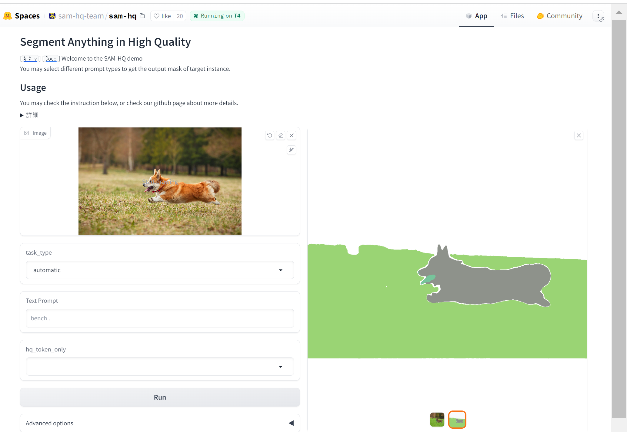
- HQ-SAM (ゼロショットのセグメンテーション)のオンラインデモ(Google Colaboratory 上): https://colab.research.google.com/drive/1QwAbn5hsdqKOD5niuBzuqQX4eLCbNKFL?usp=sharing
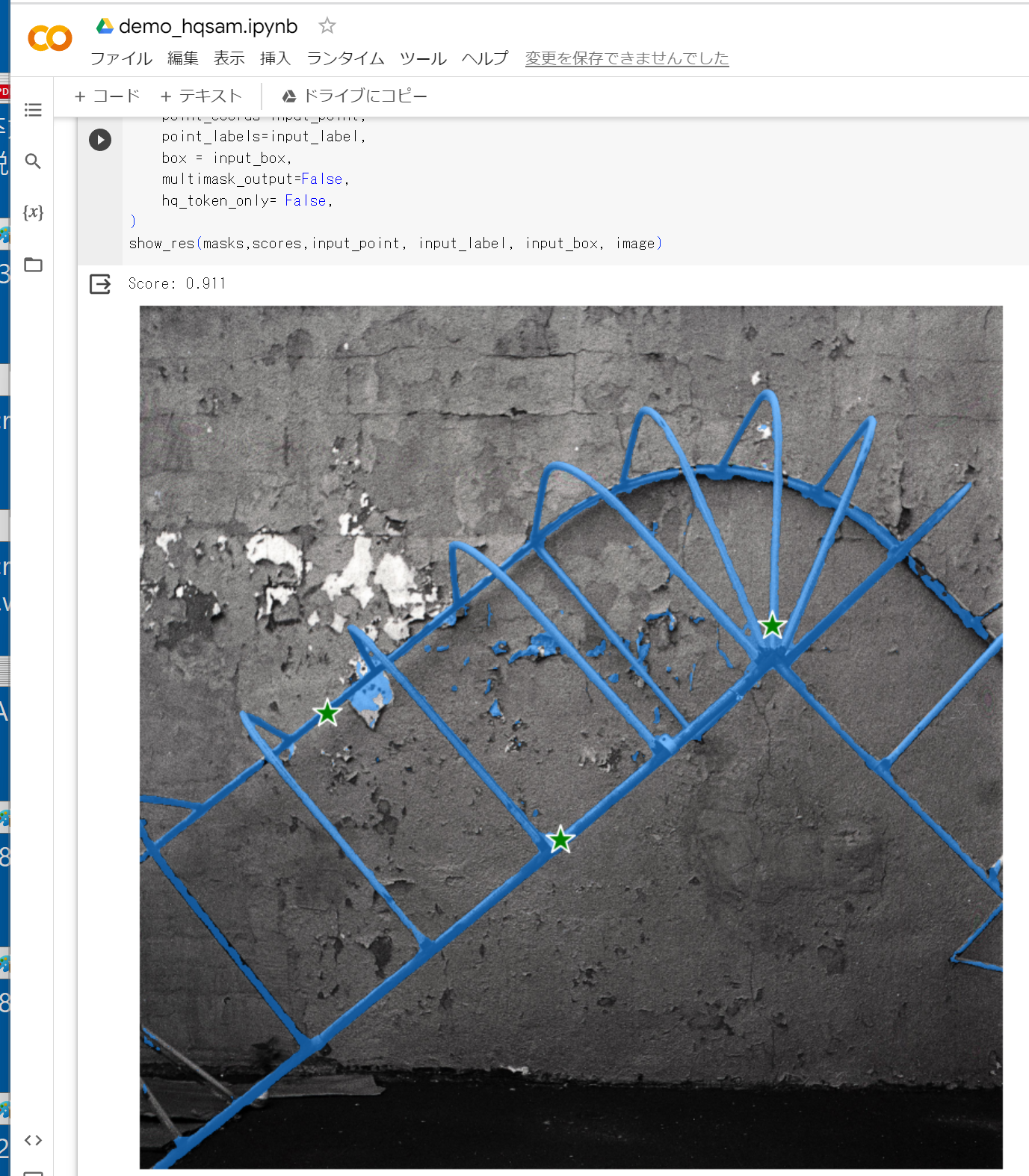
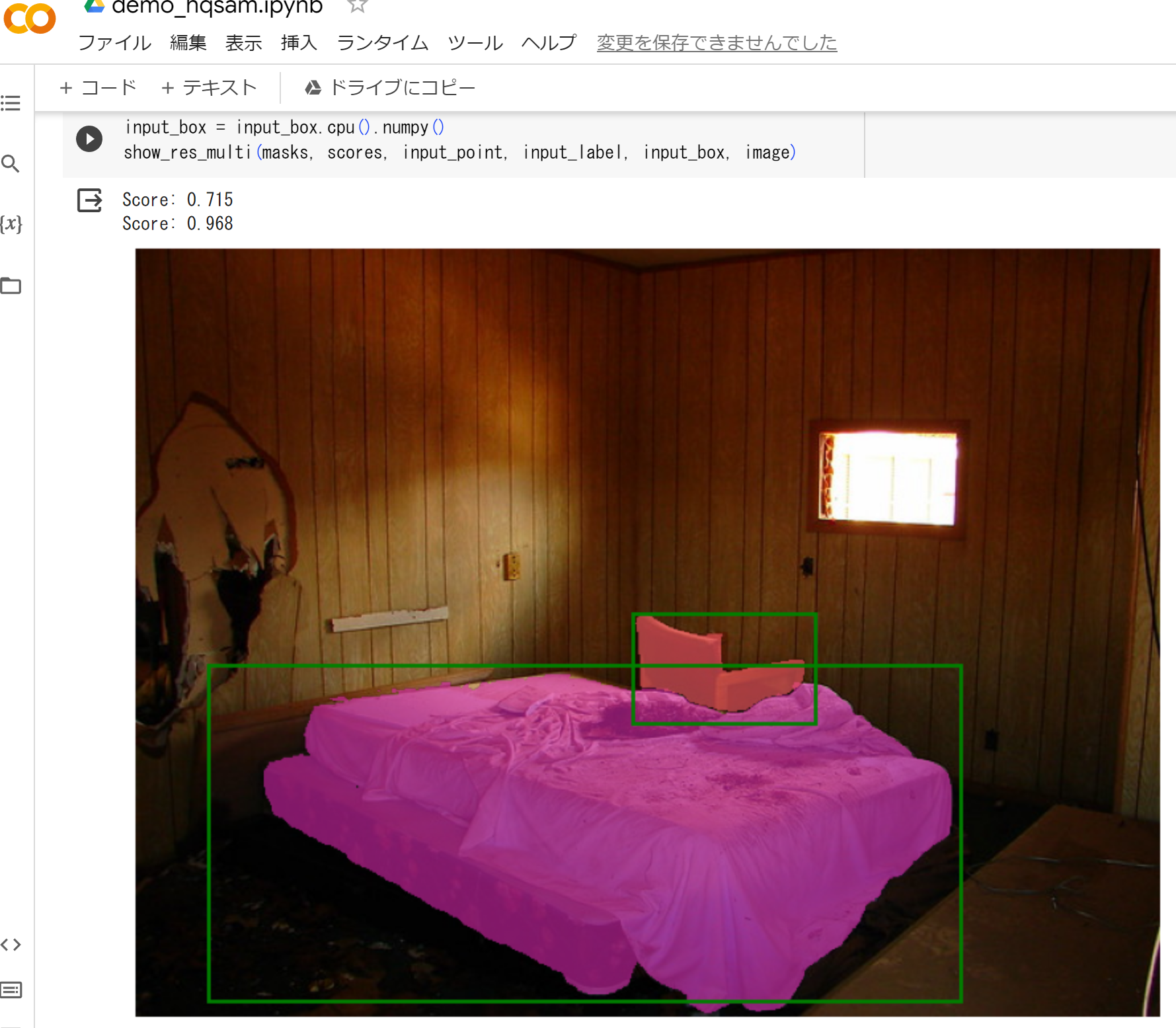
- Papers with Code のページ: https://paperswithcode.com/paper/segment-anything-in-high-quality
【関連項目】 SAM (Segment Anything Model)
HRNetw32
姿勢推定 (pose estimation) の一手法である.
【関連項目】 MMPose, 姿勢推定 (pose estimation)
Human 3.6M データセット
ディープラーニングにより姿勢推定を行うためのデータとして利用できる.
利用には, https://vision.imar.ro/human3.6m/register.php での申請を必要とする.
http://vision.imar.ro/human3.6m/description.php
Catalin Ionescu, Dragos Papava, Vlad Olaru and Cristian Sminchisescu, Human3.6M: Large Scale Datasets and Predictive Methods for 3D Human Sensing in Natural Environments, IEEE Transactions on Pattern Analysis and Machine Intelligence, vol. 36, No. 7, July 2014
iBUG 300-W データセット
iBUG 300-W データセットは, 顔の 68 ランドマーク のデータである.7764枚の顔画像について,手作業で,顔の 68 ランドマークのアノテーションとラベル付けが行われている.
顔ランドマーク (facial landmark)は,目,眉,鼻,口,あごのラインなど,顔のパーツの構造を特定できる形状予測器 (shape predictor) の学習に使うことができる.
iBUG 300-W データセットの URL: https://ibug.doc.ic.ac.uk/resources/300-W/
【関連項目】 顔の 68 ランドマーク, 顔ランドマーク (facial landmark), 顔のデータベース
image content removal(画像コンテンツの除去)
画像の中で,除去する対象となるオブジェクトの境界などを指定することにより, 指定されたオブジェクトを除去し,除去された部分の画素は, image completion and extrapolation で補う.
次の文献では, 除去する対象となるオブジェクトの境界を正確に指定しなくても, オブジェクトスコアマップ (object score map) を scene parsing network を用いて 推定することにより, image content removal(画像コンテンツの除去)ができるとされている.
- Huang JB, Kang SB, Ahuja N, Kopf J, Image completion using planar structure guidance, ACM Transactions on Graphics (TOG), 2014.
https://github.com/SunskyF/StructCompletion-python
実行の前準備として,「pip install -U opencv-python opencv-contrib-python」を実行する.demo.py の実行結果は次の通りである.
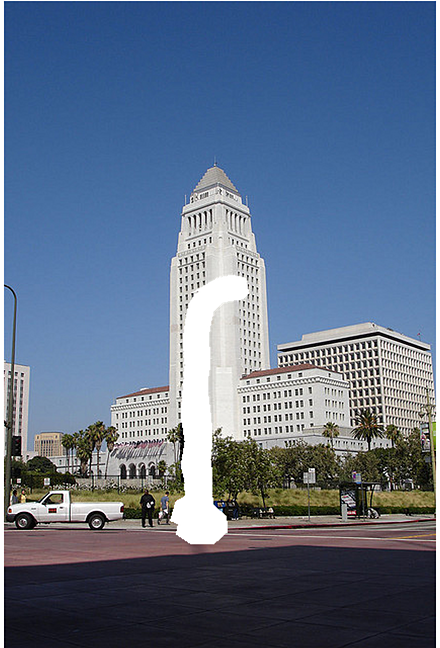
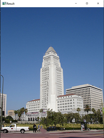
【関連項目】 image completion and extrapolation
image matting
前景の色を F,背景の色を B とし,元画像の色は I = alpha * F + (1 - alpha) * B とする. 元画像 I は既知であり,F, B, alpha は未知であるとする. このとき alpha を推定することを image matting という(alpha image matting ともいう).
写真や動画の前景背景分離に用いることができる. 物体検出 や salient object detection との違いとしては, ガラスなどの半透明なもの,髪の毛や網のようなもの,そして,前景が必ずしも画面中央に集まっているとは限らず,画面全域にある(網越しに外を見るような場合)を想定していることがある.
【関連情報】
- Papers with Code の image matting のページ: https://paperswithcode.com/task/image-matting
【関連項目】 GCA, IndexNet, DIM, AIM-500 (Automatic Image Matting-500) データセット
Trimap-based matting
trimap では,次の 3つを考える. 前景である画素は白,背景である画素は黒,transition である画素は灰色の 3通りに 塗り分けた画像を trimap という.
- 前景 (foreground)
- 背景 (background)
- transition: どちらであるか判断できないか,細かすぎて,塗り分けが困難な領域
Trimap-based matting では, 元画像と,その trimap を用いて image matting を行う. ディープラーニングによる Trimap-based matting の手法としては,Xu らの Deep Image Matting (DIM) (2017年)(文献 [1])などが知られている.
【関連情報】
- 文献 [1], Xu らの Deep Image Matting (DIM)
Ning Xu, Brian Price, Scott Cohen, Thomas Huang, Deep Image Matting, CVPR 2017, CoRR, https://arxiv.org/abs/1703.03872v3
Background matting
Background matting は,image matting において背景画像を用いる. つまり,元画像と,追加の背景画像を用いて image matting を行う. 元画像での背景と,追加の背景画像は同一の場所で撮影されたものが想定されている.そのとき,完全に一致しなくてもよい(わずかな位置のずれや照明条件の変化は許容される).
ディープラーニングによる background matting としては, Shanchuan Lin らの Background Matting(2021年)(文献 [2])などが知られる. Backbone に ResNet50, ASPP (Atrous Spatial Pyramid Pooling, DeepLabv3 のものに従う)を使用している.
Background matting では,Trimap を必要としない. ZOOM などのビデオ会議などで,グリーンバックを使わずに,前景と背景を分離するとき, 背景の取得は容易であり, Background matting は有用である.
【関連情報】
- 文献 [2], Shanchuan Lin らの Background Matting
Shanchuan Lin, Andrey Ryabtsev, Soumyadip Sengupta, Brian Curless, Steve Seitz, Ira Kemelmacher-Shlizerman, Real-Time High-Resolution Background Matting, CVPR 2021, also CoRR, abs/2012.07810v1, 2021.
https://arxiv.org/pdf/2012.07810v1.pdf
Portrait matting
人物や動物に特化した image matting である. 人物や動物が写った写真や動画に対して,image matting を行う. このとき,Trimap や背景画像などの追加の情報を準備することなく image matting を行う手法が種々提案されている.
Automatic image matting
Trimap や背景画像などの追加の情報を必要とせず, 人物や動物など以外でも(例えば,半透明のコップ,網越しの風景写真など)image matting を行うものである. Li らの GFM(文献 [3])(2020 年)は,ディープラーニングによる Trimap の推定が行われており, Li らの unified semantic model(文献 [4])(2021 年)は,Salient Opaque, Salient Transparent/Meticulous, Non-Salient の 3種類の画像を扱えるモデルであり,GFM の拡張により,unified semantic model の推定を行っている.
- 文献 [3]
Jizhizi Li, Jing Zhang, Stephen J Maybank, and Dacheng Tao. End-to-end animal image matting. arXiv preprint arXiv:2010.16188, 2020.
- 文献 [4]
Jizhizi Li, Jing Zhang and Dacheng Tao, Deep Automatic Natural Image Matting, 2021. https://arxiv.org/pdf/2107.07235v1.pdf
ImageNet データセット
ImageNet データセットは,画像分類や物体検出のタスクで利用されるデータセットである. 機械学習における画像分類や物体検出のタスクで,学習,検証,テストに利用される. ImageNet-1K は ImageNet データセットのサブセットで,ImageNet Large Scale Visual Recognition Challenge(ILSVRC)のベンチマークで使用されている.
- 画像の総数: 14,197,122枚(ImageNet-1K では約120万枚)
- クラス数: 約20,000種類(ImageNet-1K では1000種類),さまざまな種類を網羅
- ラベル付き画像:
画像が,ある特定のクラスのオブジェクトを含んでいるか(「有」,「無」の二値)
- 物体検出のアノテーション
画像内(ImageNet-1K では約45万枚)のオブジェクト(ImageNet-1K では約150万以上)の位置と大きさ(中心の座標,幅,高さ),クラス
- 画像情報:画像のサムネイルと URL.URL を使用して画像をダウンロードする場合,各画像の利用条件を利用者が確認すること.
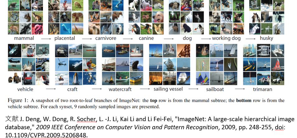
【プログラム】
ImageNet-1K の 1000クラスの表示
このプログラムは ImageNet-1K の1000クラスのデータファイル(クラス番号とクラス名のデータファイル)をダウンロードし,JSON に変換して保存した後,クラス番号とクラス名をすべて表示する.インターネット接続が必要で,requests ライブラリが必要である.
import requests
import json

def download_file(url, filename):
    """指定されたURLからファイルをダウンロードし、ローカルに保存する"""
    response = requests.get(url)
    with open(filename, 'wb') as file:
        file.write(response.content)

def convert_txt_to_json(txt_file, json_file):
    """テキストファイルをJSON形式に変換し、保存する"""
    imagenet_classes = {}
    with open(txt_file, "r") as f:
        for i, line in enumerate(f):
            imagenet_classes[str(i)] = line.strip()
    with open(json_file, "w") as f:
        json.dump(imagenet_classes, f)

def display_classes(json_file):
    """JSONファイルからクラス情報を読み込み、表示する"""
    with open(json_file) as f:
        imagenet_classes = json.load(f)
    for class_id, class_name in imagenet_classes.items():
        print(f"Class ID: {class_id}, Class Name: {class_name}")

# メイン処理
if __name__ == "__main__":
    url = "https://raw.githubusercontent.com/pytorch/hub/master/imagenet_classes.txt"
    txt_filename = "imagenet_classes.txt"
    json_filename = "imagenet_class_index.json"
    # ファイルのダウンロード
    download_file(url, txt_filename)
    # テキストファイルをJSONに変換
    convert_txt_to_json(txt_filename, json_filename)
    # クラス情報の表示
    display_classes(json_filename)
ImageNet のクラス: 別ファイルに記載している.
ImageNet データセットは次の URL で公開されているデータセット(オープンデータ)である.
ImageNet データセットの URL: https://image-net.org/
【関連する外部ページ】
- 文献: abs/1409.0575
- Papers With Code の ImageNet データセットのページ: https://paperswithcode.com/dataset/imagenet
- PyTorch の ImageNet データセット: https://pytorch.org/vision/stable/datasets.html#imagenet
- TensorFlow データセットの imagenet2012 データセット: https://www.tensorflow.org/datasets/catalog/imagenet2012
IMDb データセット
IMDb の URL: https://www.imdb.com/
IMDb での映画の批評は,批評文とスコア(10点満点)である. IMDb データセットでは,7点以上の批評は positive,4点以下の批評は negative としている.つまり,2種類ある. そして,IMDb データセットには,positive か negative の批評のみが含まれている(中間の点数である 5点,6点のものは含まれていない).そして, positive,negative の批評が同数である. 学習用として,positive,negative がそれぞれ 25000. 検証用として,positive,negative がそれぞれ 25000.
IMDb データセットのURL: https://ai.stanford.edu/%7Eamaas/data/sentiment/
【関連項目】 Keras に付属のデータセット, TensorFlow データセット, オープンデータ
Python での IMDb データセットのロード(TensorFlow データセットを使用)
次の Python プログラムは,TensorFlow データセットから,IMDb データセットのロードを行う. x_train, y_train が学習用のデータ.x_test, y_test が検証用のデータになる.
- x_train: 25000個のテキスト
- y_train: 25000個の数値
- x_test: 25000個のテキスト
- y_test: 25000個の数値
次のプログラムでは,ロードと確認表示を行う.
tensorflow_datasets の loadで, 「batch_size = -1」を指定して,一括読み込みを行っている.
from __future__ import absolute_import, division, print_function, unicode_literals
import tensorflow as tf
import numpy as np
import tensorflow_datasets as tfds

%matplotlib inline
import matplotlib.pyplot as plt
import warnings
warnings.filterwarnings('ignore')   # Suppress Matplotlib warnings

imdb_reviews, imdb_reviews_metadata = tfds.load('imdb_reviews', with_info = True, shuffle_files=True, as_supervised=True, batch_size = -1)
x_train, y_train, x_test, y_test = imdb_reviews['train'][0], imdb_reviews['train'][1], imdb_reviews['test'][0], imdb_reviews['test'][1]

# 確認表示
import pandas as pd
display(pd.DataFrame(x_train[0:14], y_train[0:14]))
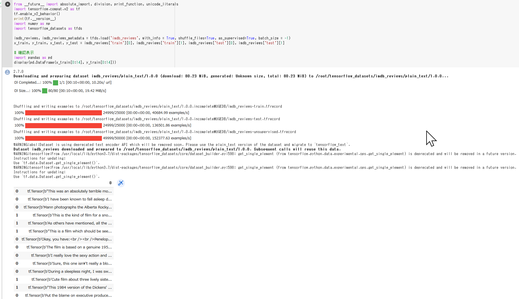
Python での IMDb データセットのロード(Keras を使用)
IMDb データセットは,次のプログラムでロードできる.
from tensorflow.keras.datasets import imdb
(x_train, y_train), (x_test, y_test) = imdb.load_data()
Imm 顔データベース (IMM Face Database)
40種類の人間の顔を撮影した240枚の画像. 58個の顔ランドマークが付いている.
URL: http://www2.imm.dtu.dk/pubdb/pubs/3160-full.html
M. M. Nordstrøm and M. Larsen and J. Sierakowski and M. B. Stegmann, The IMM Face Database - An Annotated Dataset of 240 Face Images
http://www2.imm.dtu.dk/pubdb/edoc/imm3160.pdf
【関連項目】 顔のデータベース
iNaturalist データセット
画像のデータセット.アノテーションとしてバウンディングボックスが付けられている.Imbalance の大きさを特徴とする.
次の URL で公開されているデータセット(オープンデータ)である.
URL: https://github.com/visipedia/inat_comp/tree/master/2017
- クラス数: 5,089
- 学習と検証 (validation) 用の 675,000 枚の画像.テスト用の 183,000 枚の画像.
- バウンディングボックス数: 183,000
- Imbalance 値: 453.44
- 文献
Grant Van Horn, Oisin Mac Aodha, Yang Song, Yin Cui, Chen Sun, Alex Shepard, Hartwig Adam, Pietro Perona, Serge Belongie, The iNaturalist Species Classification and Detection Dataset, CVPR 2018, 2018.
- Papers with Code のページ: https://paperswithcode.com/dataset/inaturalist
- TensorFlow のモデル: https://github.com/tensorflow/models
InsightFace
顔検出 (face detection),顔のアラインメント, 顔検証 (face verification), 顔識別 (face identification)の機能を持つ.
- 顔検出 (face detection): RetinaFace, SCRFD, blazeface_paddle をサポートしている.
InsightFace の GitHub のページ: https://github.com/deepinsight/insightface
【関連項目】 ArcFace 法, Chandrika Deb の顔マスク検出, Dlib の顔検出, face alignment, MobileFaceNets, 顔検出 (face detection)
Google Colaboratory で,InsightFace による顔検出及び年齢と性別の予測
公式ページ (https://github.com/deepinsight/insightface/tree/master/python-package) に記載の顔検出及び年齢と性別の予測のプログラムを変更して実行する.
このプログラムは buffalo_l という名前の事前学習済みモデルを使用している.
- 顔検出のモデル: SCRFD-10GF
- 顔認識のモデル: ResNet50@WebFace600K
- 顔のアラインメント: 2d106, 3d68
- 属性: 年齢,性別
次のコマンドやプログラムは Google Colaboratory で動く(コードセルを作り,実行する).
- InsightFace のインストール
GPU を使わない場合には「onnxruntime-gpu」でなく,「onnxruntime」をインストールすること.
!pip3 install -U insightface onnxruntime-gpu opencv-python numpy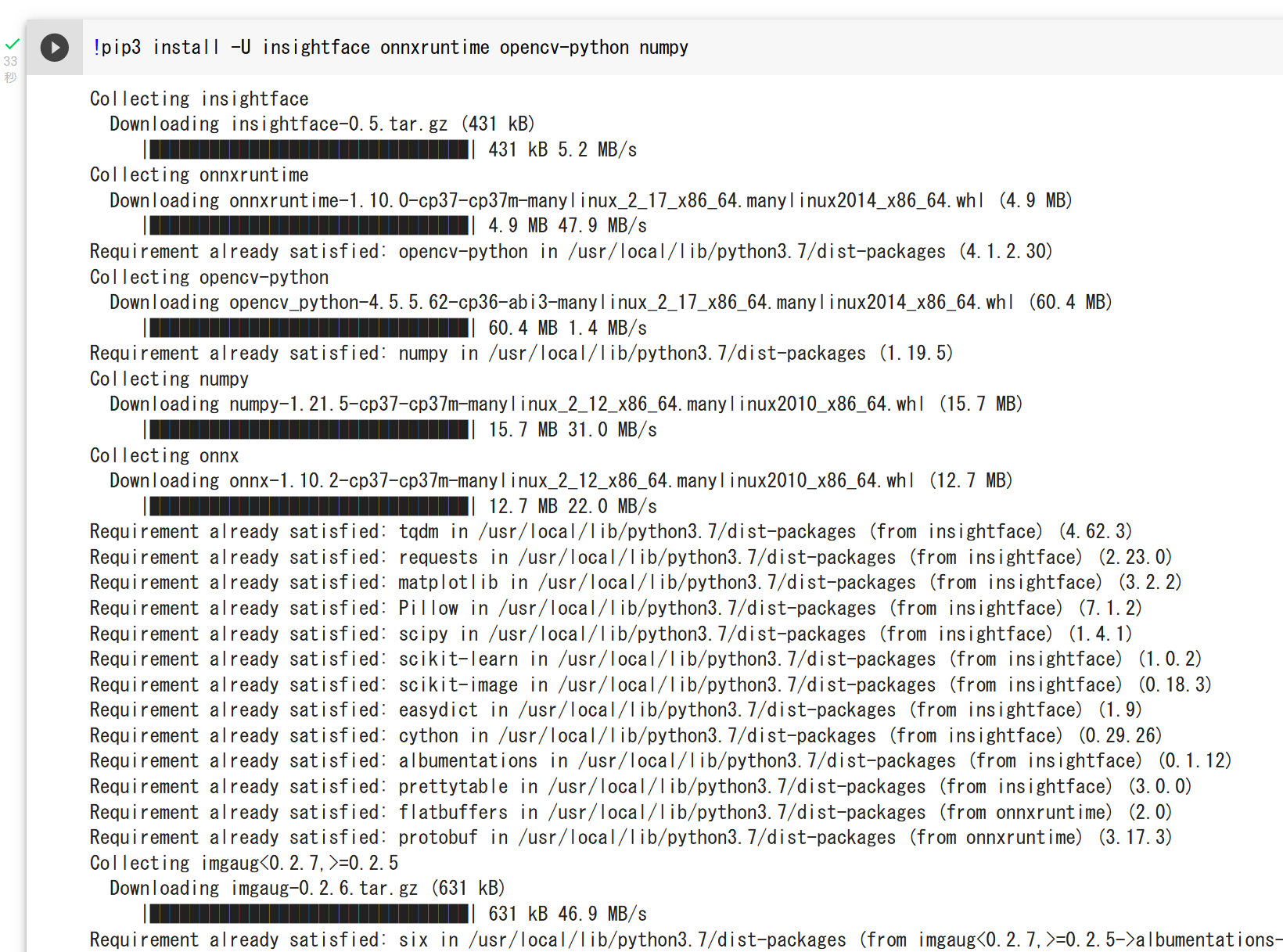
- 顔検出及び年齢と性別の予測の実行(サンプル画像を使用)
動作確認のため,公式ページ (https://github.com/deepinsight/insightface/tree/master/python-package) に記載の,顔検出及び年齢と性別の予測のプログラムを実行する.
このプログラムは buffalo_l という名前の事前学習済みモデルを使用している.- 顔検出のモデル: SCRFD-10GF
- 顔認識のモデル: ResNet50@WebFace600K
- 顔のアラインメント: 2d106, 3d68
- 属性: 年齢,性別
このプログラムの実行により,result.jpg ファイルができる.
import cv2
import numpy as np
%matplotlib inline
import matplotlib.pyplot as plt
import warnings
warnings.filterwarnings('ignore')   # Suppress Matplotlib warnings
import insightface
from insightface.app import FaceAnalysis
from insightface.data import get_image as ins_get_image

app = FaceAnalysis(providers=['CUDAExecutionProvider', 'CPUExecutionProvider'])
app.prepare(ctx_id=0, det_size=(640, 640))

img = ins_get_image('t1')
faces = app.get(img)
rimg = app.draw_on(img, faces)
for i in faces:
  print("gender %s, age %d" % (('F' if i['gender'] == 0 else 'M'), i['age']))
plt.style.use('default')
plt.imshow(cv2.cvtColor(rimg, cv2.COLOR_BGR2RGB))
plt.show()
cv2.imwrite("./result.jpg", rimg)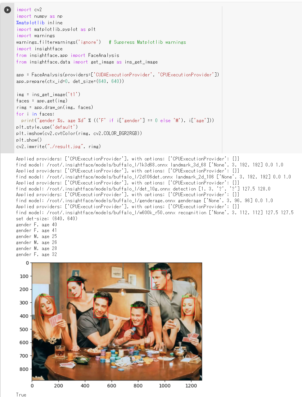
- 顔検出及び年齢と性別の予測の実行(任意の画像ファイルを使用)
顔の画像ファイルは何でも良いが,ここでは,画像ファイルをダウンロードしている.
!curl -O https://www.kkaneko.jp/sample/face/3284.png
!curl -O https://www.kkaneko.jp/sample/face/3285.png
!curl -O https://www.kkaneko.jp/sample/face/3287.png
!curl -O https://www.kkaneko.jp/sample/face/3288.png
!curl -O https://www.kkaneko.jp/sample/face/3289.png
!curl -O https://www.kkaneko.jp/sample/face/3290.png
いま準備した画像ファイルについて,顔検出及び年齢と性別の予測を実行する.
import cv2
import numpy as np
%matplotlib inline
import matplotlib.pyplot as plt
import warnings
warnings.filterwarnings('ignore')   # Suppress Matplotlib warnings
import insightface
from insightface.app import FaceAnalysis
from insightface.data import get_image as ins_get_image

app = FaceAnalysis(providers=['CUDAExecutionProvider', 'CPUExecutionProvider'])
app.prepare(ctx_id=0, det_size=(640, 640))

files = ['3284.png', '3285.png','3287.png', '3288.png', '3289.png', '3290.png']

for f in files:
    img = cv2.imread(f)
    faces = app.get(img)
    for i in faces:
        print("gender %s, age %d" % (('F' if i['gender'] == 0 else 'M'), i['age']))
    rimg = app.draw_on(img, faces)
    plt.style.use('default')
    plt.imshow(cv2.cvtColor(rimg, cv2.COLOR_BGR2RGB))
    plt.show()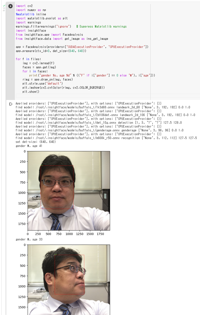
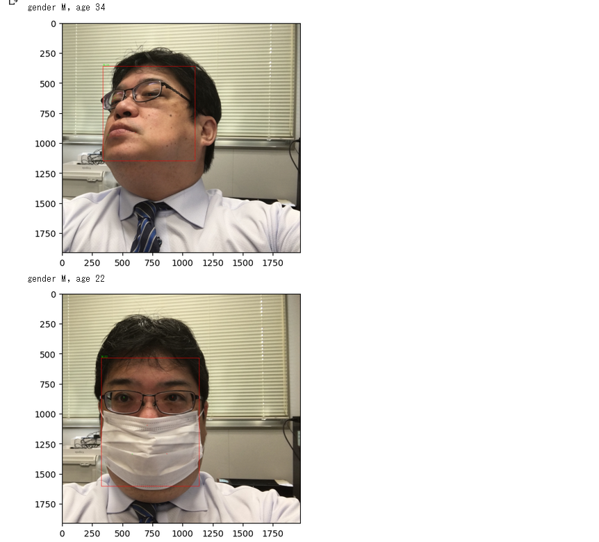
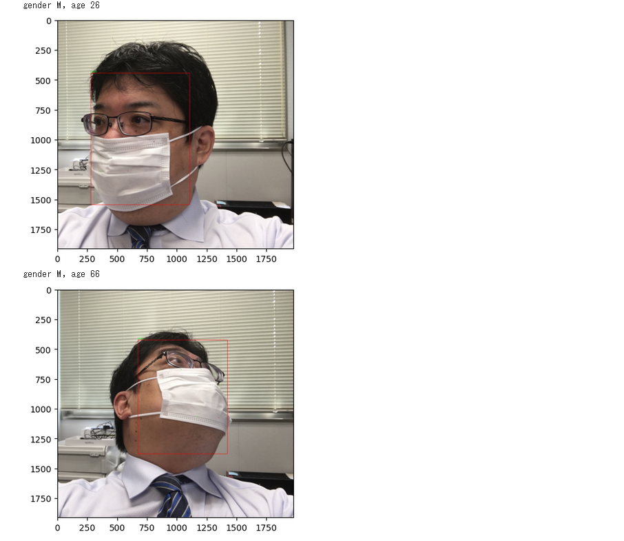
顔検出,年齢と性別の推定,顔識別,人体検出(InsightFace のインストールと動作確認)(PyTorch,Python を使用)(Windows 上)
別ページ »で説明
InsightFace のインストールと動作確認(顔検出,年齢と性別の推定)(Python, PyTorch を使用)(Ubuntu 上)
別ページ »で説明
Iris データセット
Iris データセットは公開されているデータセット(オープンデータ)である.
- 行数: 150行
- 属性: sepal length, sepal width, petal length, petal width, species
【文献】
R.A. Fisher, The use of multiple measurements in taxonomic problems, Annual Eugenics, 7, Part II, pp. 179-188, 1936.
【サイト内の関連ページ】
- Iris データセットについての説明資料: iris.pdf [PDF], [パワーポイント]
- Iris データセットを扱う Python プログラム: 別ページ で説明している.
【関連する外部ページ】
JHU-CROWD++ データセット
画像数は 4,822枚である. 各画像の人物数は 0 から 25,791 である.
- 文献
Vishwanath A. Sindagi, Rajeev Yasarla, and Vishal M. Patel, JHU-CROWD++: Large-Scale Crowd Counting Dataset and A Benchmark Method, IEEE Transactions on Pattern Analysis and Machine Intelligence, 2020.
- 公式ページ: http://www.crowd-counting.com/
【関連項目】 crowd counting, FIDTM, オープンデータ
Keras
Keras は 機械学習のAPI の機能を持つ. Python 言語から利用可能. TensorFlow, CNTK, Theano など,さまざまなディープラーニングのフレームワークの上で動く.
Keras の概要
- Keras のモデルは,複数の層が組み合わさったもの.単純に層を積み重ねたもの(シーケンシャル)や,複雑な構成のもの(グラフ)がある
- Keras の層には,活性化関数,層の種類(カーネル,バイアスなど)を設定できる
- Keras の層には,全結合層,畳み込み(コンボリューション)層などの種類がある
- 学習のために,オプティマイザの設定を行う
- Keras のモデルの構成やオプティマイザの設定は,保存できる
- 学習の結果は,重みになる. チェックポイントにより,重みも保存できる.
次のプログラムでは,損失関数を sparse_categorical_crossentropy, 最適化法を 確率的勾配降下法 (SGD 法), 尺度を accuracy に設定している.
m.compile(optimizer=tf.keras.optimizers.SGD(lr=0.01, momentum=0.9, nesterov=True),
          loss='sparse_categorical_crossentropy',
          metrics=['accuracy'])
目的関数については: https://keras.io/ja/objectives/
【関連する外部ページ】
- URL: https://keras.io/ja/
- GitHub: https://github.com/fchollet/keras
- Keras 応用: https://keras.io/api/applications/
【サイト内の関連ページ】
- Windows でのインストール詳細(NVIDIA ドライバ,NVIDIA CUDA ツールキット,NVIDIA cuDNN, TensorFlow 関連ソフトウェアを含む): 別ページ »で説明
- Ubuntu でのインストール詳細(NVIDIA ドライバ,NVIDIA CUDA ツールキット,NVIDIA cuDNN, TensorFlow 関連ソフトウェアを含む): 別ページ »で説明
【関連項目】 Applications of Deep Neural Networks, TensorFlow, ディープラーニング
Keras のインストール
- Windows でのインストール詳細(NVIDIA ドライバ,NVIDIA CUDA ツールキット,NVIDIA cuDNN, TensorFlow 関連ソフトウェアを含む): 別ページ »で説明
- Ubuntu でのインストール詳細(NVIDIA ドライバ,NVIDIA CUDA ツールキット,NVIDIA cuDNN, TensorFlow 関連ソフトウェアを含む): 別ページ »で説明
Keras-GAN のページ
Erik Linder-Norén により GitHub で公開されているKeras-GAN のページ.
URL は次の通り.
Keras-GAN のページ: https://github.com/eriklindernoren/Keras-GAN
Keras でのカーネルの初期化
次のプログラムの中の kernel_initializer の部分. 標準偏差を 0.01 になるように重みを設定している.
m.add(Dense(units=100, input_dim=768, kernel_initializer=tf.keras.initializers.TruncatedNormal(stddev=0.01)))
Keras での学習
教師データ x_train と y_train (x_train は入力データの numpy 配列もしくは numpy 配列のリスト,y_train はクラス番号の numpy 配列)を用いて, バッチサイズが 32,エポック数を 50 として学習したいときには,次のコマンドを用いる.
history = m.fit(x_train, y_train, batch_size=32, epochs=50, validation_data=(x_test, y_test))
Keras での検証(バリデーション)
Keras での学習において,「validation_data」を付けることで,検証(バリデーション)が行われる.
このとき,検証(バリデーション)に使うデータ(x_test, y_test)をいろいろ変えながら,Kerasでの検証(バリデーション)を行う.
history = m.fit(x_train, y_train, batch_size=32, epochs=50, validation_data=(x_test, y_test))
結果(上のプログラムでは history)を見て,過学習や学習不足を判断する.history は次のようなプログラムで表示できる.
import pandas as pd
h = pd.DataFrame(history.history)
h['epoch'] = history.epoch
print(h)
Keras でのコンパイル
Keras のモデルのコンパイルにおいては, オプティマイザ(最適化器)と 損失関数とメトリクスの指定を行う必要がある.
Keras でのモデル m のコンパイルのプログラムは「m.compile」のように書く.
Keras に付属のデータセット
データセットは,データの集まりのこと. Python の keras には,次のデータセットを簡単にダウンロードできる機能がある.
- CIFAR-10 データセット: カラー画像 60000枚, カテゴリーラベル (category label)
CIFAR-10 データセットは,次のプログラムでロードできる.
【Keras のプログラム】from tensorflow.keras.datasets import cifar10 (x_train, y_train), (x_test, y_test) = cifar10.load_data() - CIFAR-100 データセット: カラー画像 60000枚, カテゴリーラベル (category label)
CIFAR-100 データセットは,次のプログラムでロードできる.
【Keras のプログラム】from tensorflow.keras.datasets import cifar100 (x_train, y_train), (x_test, y_test) = cifar100.load_data(label_mode='fine') - IMDb データセット: 25000 の映画レビュー
IMDb データセットは,次のプログラムでロードできる.
【Keras のプログラム】from tensorflow.keras.datasets import imdb (x_train, y_train), (x_test, y_test) = imdb.load_data() - Reuters newswire topics データセット: ニュースワイヤ 11228, ラベル
Reuters newswire topics データセットは,次のプログラムでロードできる.
【Keras のプログラム】from tensorflow.keras.datasets import reuters (x_train, y_train), (x_test, y_test) = reuters.load_data() - MNIST データセット: 濃淡画像 70000枚, ラベル
MNIST データセットは,次のプログラムでロードできる.
【Keras のプログラム】from tensorflow.keras.datasets import mnist (x_train, y_train), (x_test, y_test) = mnist.load_data() - Fashion MNIST データセット: 濃淡画像 70000枚, ラベル
Fashion MNIST データセットは,次のプログラムでロードできる.
【Keras のプログラム】from tensorflow.keras.datasets import fashion_mnist (x_train, y_train), (x_test, y_test) = fashion_mnist.load_data() - Boston housing price 回帰データセット: 13属性
Boston housing price 回帰データセットは,次のプログラムでロードできる.
【Keras のプログラム】from tensorflow.keras.datasets import boston_housing (x_train, y_train), (x_test, y_test) = boston_housing.load_data()
keras に付属のデータセットを取得するときのオプションについては, https://keras.io/ja/datasets/(日本語版), https://keras.io/api/datasets/(英語版) に説明されている.
【関連項目】 Boston housing price 回帰データセット, CIFAR-10 データセット, CIFAR-100 データセット, IMDb データセット, Reuters newswire topics データセット, MNIST データセット, Fashion MNIST データセット
Keras の応用
Keras の応用としては, MobileNetV2, Inception-ResNet, ResNet50, DenseNet121, DenseNet169, NASNetなどの画像分類のモデルがある. (その詳細は,https://keras.io/ja/applications/)
Keras では,これらモデルについて,ImageNet データセット での学習済みモデルを,次のようなプログラムで,簡単に使えるようにすることができる.
from tensorflow.keras.applications.mobilenet_v3 import MobileNetV3
m = MobileNetV3(weights='imagenet')
【関連項目】 ResNet50, ResNet101, ResNet152, その他の ResNet, Inception-ResNet, DenseNet121, DenseNet169, NASNet, MobileNetV2
Keras で利用可能な画像分類のモデルは,https://keras.io/api/applications/index.html で説明されている.
Kinetics Human Action Video Dataset (Kinetics Human Action Video データセット)
400/600/700 種類の人間の行動をカバーする最大65万のビデオクリップの URL リンク集とアノテーションである. それぞれのクリップには,1つの行動クラスがアノテーションされている. ビデオの長さは,約10秒である. 機械学習による行動分類,行動認識,ビデオ検索などの学習や検証に利用できるデータセットである.
ディープラーニングで,人間の行動推定に利用できる.
- 約65万のビデオクリップのURLリンク
- 楽器の演奏などの人間と物体のインタラクション,握手やハグなどの人間と人間のインタラクションを網羅
- 行動クラスの数は 400/600/700
- 各ビデオクリップには1つの行動クラスがアノテーションされている.
- 各ビデオクリップの長さは約10秒である.
Kinetics データセットは次の URL で公開されているデータセット(オープンデータ)である.
https://deepmind.com/research/open-source/kinetics
【関連情報】
- URL: http://human-pose.mpi-inf.mpg.de/
- URL: https://deepmind.com/research/open-source/kinetics
- 文献
W. Kay, J. Carreira, K. Simonyan, B. Zhang, C. Hillier, S. Vijayanarasimhan, F. Viola, T. Green, T. Back, P. Natsev, M. Suleyman, and A. Zisserman. The kinetics human action video dataset. arXiv preprint arXiv:1705.06950, 2017.
- Papers With Code の Kinetics データセットのページ: https://paperswithcode.com/dataset/kinetics
- PyTorch の Kinetics データセット: https://pytorch.org/vision/stable/datasets.html#torchvision.datasets.Kinetics400
Google Colaboratory で,Kinetics データセットのダウンロード
次のコマンドは Google Colaboratory で動く(コードセルを作り,実行する).
!curl -O https://storage.googleapis.com/deepmind-media/Datasets/kinetics700_2020.tar.gz
!tar -xvzf kinetics700_2020.tar.gz
!ls kinetics700_2020
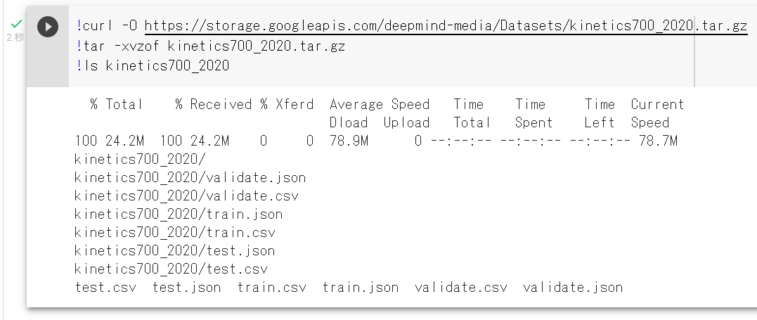
Windows での Kinetics データセットのダウンロード
Windowsで次のように操作する.
mkdir c:\data
mkdir c:\data\kinetics
cd c:\data\kinetics
curl -O https://storage.googleapis.com/deepmind-media/Datasets/kinetics700_2020.tar.gz
"c:\Program Files\7-Zip\7z.exe" x kinetics700_2020.tar.gz
"c:\Program Files\7-Zip\7z.exe" x kinetics700_2020.tar
KITTI データセット
カラーのカメラ,モノクロのステレオカメラ,3次元レーザースキャナなどのさまざまなセンサーのデータから構成される.
- 数時間分の交通シナリオ
- セマンティック・セグメンテーションのグランドトゥルースが含まれているわけではない
http://www.cvlibs.net/datasets/kitti
【関連情報】
- A. Geiger, P. Lenz and R. Urtasun, "Are we ready for autonomous driving? The KITTI vision benchmark suite," 2012 IEEE Conference on Computer Vision and Pattern Recognition, 2012, pp. 3354-3361, doi: 10.1109/CVPR.2012.6248074.
- Papers With Code の KITTI データセットのページ: https://paperswithcode.com/dataset/kitti
- PyTorch の KITTI データセット: https://pytorch.org/vision/stable/datasets.html
- TensorFlow データセット の KITTI データセット: https://www.tensorflow.org/datasets/catalog/kitti
KITTI オドメトリデータセットのダウンロード
車両からの観測画像と車両の自己位置のデータ.ビジュアルオドメトリに使用する.
URL: https://github.com/uoip/monoVO-python
- テスト用の画像データのダウンロードと展開(解凍)
テスト画像データをダウンロードする.uoip / monoVO-python の Web ページを開く.
- 「KITTI odometry data set (grayscale, 22 GB)」をクリックする.
- 濃淡 (grayscale) 画像が欲しいので,「Download odometry data set (grayscale, 22GB)」をクリックする.
これは,画像データの .zip ファイルである(多数の .png形式の画像ファイルを zip 形式に固めたものである).
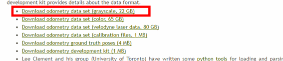
- メールアドレスを登録し,「Request Download Link」をクリックする.
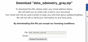
- 電子メールで通知が送られてくるので確認の上,電子メールの中のリンクをクリックする.
- 件名を確認し,他のメールと勘違いしていないことをよく確認したうえでリンクをクリックすること.
- 通知が送られるまで,それほど時間はかからない.
- 電子メールの中身を他の人に見せる(他の人に代理作業を頼む)のはマナー違反である.
- リンクをクリックすると,ダウンロードが始まるので確認する.
ダウンロードには時間がかかる.
- いまダウンロードしたテスト用画像データの .zip ファイルを,分かりやすいディレクトリ(日本語を含まないこと)に展開(解凍)する.
この .zip ファイルは,C:\data_odometry_gray\dataset に展開(解凍)したものとして,説明を続けるので,適切に読み替えること.
- 展開(解凍)してできたファイルを確認する.
- .png 形式のファイルが多数ある
- ファイル名は6桁の数字の連番になっている
- 多数のディレクトリに分かれている
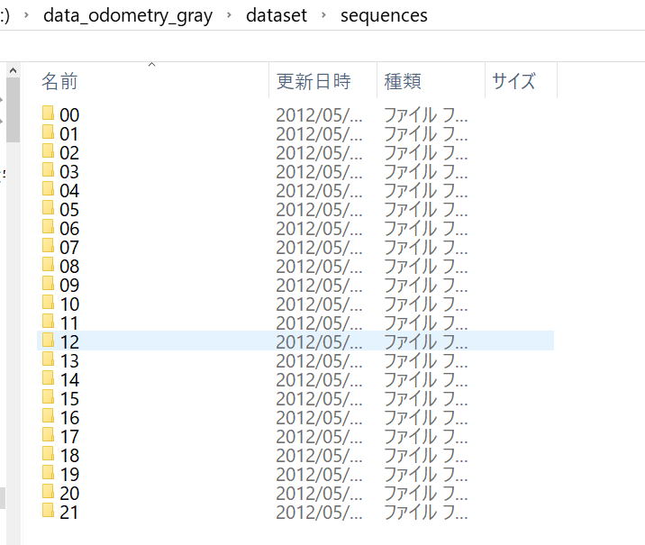
KITTI データセットのビジュアライザ
https://github.com/navoshta/KITTI-Dataset
KITTI データセットの Python インタフェース
https://github.com/utiasSTARS/pykitti
K 近傍探索 (K nearest neighbour)
K 近傍探索 (K nearest neighbour)のアルゴリズムは,次の性質を持つ.
- 事前に,データを複数準備する(事前データ).
- それぞれのデータに,ラベルが付いている.
- 新しいデータが1つあるとき,それを事前データそれぞれすべてと類似度を計算する.
- 類似度が高いもの数個を選ぶ.そして,選ばれた数個のラベルについて多数決を取る.
- その結果得られたラベルを識別結果とする.
【関連項目】 Fast-Robust-ICP, libnabo, libpointmatcher
L2 正則化
正則化の一手法である. L2 正則化では,重みの二乗の合計に比例したペナルティを,重みに与える.
L2 正則化を行いたいときは次のようにする.
import tensorflow.compat.v2 as tf
tf.keras.layers.Dense(128, activation='relu', kernel_regularizer=tf.keras.regularizers.l2(0.001))
LabelMe インタフェース
LabelMe インタフェースは,アノテーションのツールである.
- 文献
Russell BC, Torralba A, Murphy KP, Freeman WT, Labelme: a database and web-based tool for image annotation. Int'l Journal of Computer Vision, 2008.
- 公式ページ (GitHub のページ): https://github.com/wkentaro/labelme
【関連項目】 アノテーション (annotation)
Windows での LabelMe のインストールと確認
公式ページ https://github.com/wkentaro/labelmeの記載に従う.
- インストール
Windows では,コマンドプロンプトを管理者として実行し, 次のコマンドを実行する.
python -m pip install labelme - 確認のため「labelme」で起動する.
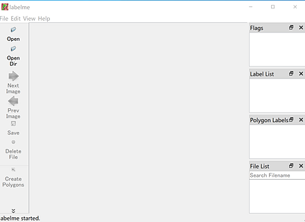
LAION
LAION-2B の画像数は約20億枚. LAION-5B の画像数は約50億枚.
【関連する外部ページ】
LAION の公式ページ: https://laion.ai/
LaMa
LaMa は,Image Inpainting(イメージ・インペインティング)のための技術である.2021年発表.
Image Inpainting(イメージ・インペインティング)とは, 画像の欠落部分を補うことであり,画像の中の不要な部分を消すときにも役立つ.
LaMa のデモページ
- LaMa のデモページの URL: https://colab.research.google.com/github/saic-mdal/lama/blob/master/colab/LaMa_inpainting.ipynb#scrollTo=-VZWySTMeGDM
- LaMa のデモページの実行結果の例
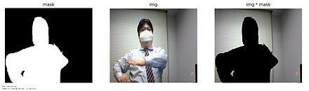
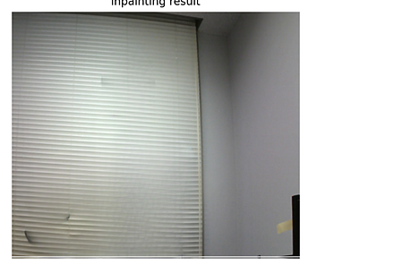
【関連項目】 image inpainting
Windows での Lama Cleaner のインストール
Windows での Lama Cleaner のインストール: 別ページで説明している.
Leeds Sports Pose Dataset (LSP データセット)
スポーツ選手を中心として,Flickr から収集した2000枚の画像に, 姿勢(ポーズ)についてのアノテーションを行ったもの. 最も目立つ人物が,およそ150ピクセルになるようにスケーリングされている. 各画像には,14個のジョイント(関節)の位置がアノテーションされている. オリジナル画像の帰属 (attribution) とFlickrのURLは,各画像ファイルのJPEGコメントに記載されている.
ディープラーニングにより姿勢推定を行うためのデータとして利用できる.
次の URL で公開されているデータセット(オープンデータ)である.
URL: https://dbcollection.readthedocs.io/en/latest/datasets/leeds_sports_pose_extended.html
【関連情報】
- 文献
Sam Johnson, and Mark Everingham. Clustered Pose and Nonlinear Appearance Models for Human Pose Estimation. In Frédéric Labrosse, Reyer Zwiggelaar, Yonghuai Liu, and Bernie Tiddeman, editors, Proceedings of the British Machine Vision Conference, pages 12.1-12.11. BMVA Press, September 2010. doi:10.5244/C.24.12.
http://www.bmva.org/bmvc/2010/conference/paper12/paper12.pdf
- Papers With Code の LSP データセットのページ: https://paperswithcode.com/dataset/lsp
- open-mmlab での記事
https://github.com/open-mmlab/mmpose/blob/master/docs/en/tasks/3d_body_mesh.md#lsp
Google Colaboratory で,Leeds Sports Pose Dataset (LSP データセット)のダウンロード
次のコマンドは Google Colaboratory で動く(コードセルを作り,実行する).
!curl -O http://sam.johnson.io/research/lsp_dataset.zip
!curl -O http://sam.johnson.io/research/lspet_dataset.zip
!unzip lsp_dataset.zip -d lsp_dataset
!unzip lspet_dataset.zip -d lspet_dataset
!ls -la lspet_dataset
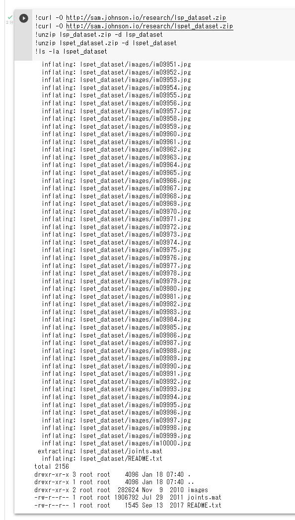
アノテーションファイルは,次の URL からダウンロードできる.
https://drive.google.com/file/d/1GZxlTLuMfA3VRvz2jyv8fhJDqElNrgKS/view
Windows での,Leeds Sports Pose Dataset (LSP データセット)のダウンロード
Windows の場合.次により c:\data\lsp にダウンロードされる.
mkdir c:\data
mkdir c:\data\lsp
mkdir c:\data\lsp\images
cd c:\data\lsp\images
curl -O http://sam.johnson.io/research/lsp_dataset.zip
curl -O http://sam.johnson.io/research/lspet_dataset.zip
powershell -command "Expand-Archive -DestinationPath . -Path lsp_dataset.zip"
powershell -command "Expand-Archive -DestinationPath . -Path lspet_dataset.zip"
アノテーションファイルは,次の URL からダウンロードできる.
https://drive.google.com/file/d/1GZxlTLuMfA3VRvz2jyv8fhJDqElNrgKS/view
Ubuntu での,Leeds Sports Pose Dataset (LSP データセット)のダウンロード
Ubuntu の場合.次により,/usr/local/data/lsp/images にダウンロードされる.
mkdir -p /usr/local/data/lsp/images
cd /usr/local/data/lsp/images
curl -O http://sam.johnson.io/research/lsp_dataset.zip
curl -O http://sam.johnson.io/research/lspet_dataset.zip
unzip lsp_dataset.zip -d lsp_dataset
unzip lspet_dataset.zip -d lspet_dataset
アノテーションファイルは,次の URL からダウンロードできる.
https://drive.google.com/file/d/1GZxlTLuMfA3VRvz2jyv8fhJDqElNrgKS/view
LFW データセット
LFWデータセットは,「in-the-wild」のラベル付きの顔のデータベースである. 合計で 13,233枚,5,749人の顔画像が含まれている.
機械学習による顔認識の学習や検証に利用できるデータセットである.
- 5,749 人の顔について,IDが付いている.
- 1,680 人については,2つ以上の画像に写っている.他の人は,1つの画像にのみ写っている.
- 文献
Gary B. Huang, Marwan Mattar, Tamara Berg, Eric Learned-Miller. Labeled Faces in the Wild: A Database for Studying Face Recognition in Unconstrained Environments. Workshop on Faces in 'Real-Life' Images: Detection, Alignment, and Recognition, Erik Learned-Miller and Andras Ferencz and Frédéric Jurie, Oct 2008, Marseille, France. inria-00321923
- E. Learned-Miller, G. B. Huang, A. RoyChowdhury, H. Li, and G. Hua. Labeled faces in the wild: A survey. In Advances in Face Detection and Facial Image Analysis, pages 189-248. Springer, 2016.
- Papers With Code の LFW データセットのページ: https://paperswithcode.com/dataset/lfw
- TensorFlow データセットの LFW データセット: https://www.tensorflow.org/datasets/catalog/lfw
【関連項目】 顔認識 (face recognition), 顔のデータベース
librosa
librosa は, 音声,音楽の機能をもった Python のパッケージである. 主な機能としては,音源分離(music source separation),スペクトログラム, 音声ファイルの読み込み,テンポ(tempo)の推定がある.
【文献】
McFee, Brian, Colin Raffel, Dawen Liang, Daniel PW Ellis, Matt McVicar, Eric Battenberg, and Oriol Nieto. "librosa: Audio and music signal analysis in python." In Proceedings of the 14th python in science conference, pp. 18-25. 2015.
【関連する外部ページ】
- 公式のドキュメントのページ: https://librosa.org/doc/latest/index.html
- 公式の GitHub のページ: https://github.com/librosa/librosa
【関連項目】 short-time Fourier transform, 音声, 音楽, sound, 音データ(sound data)
Google Colaboratory で,パワースペクトログラムの表示(librosa を使用)
次のプログラムは Google Colaboratory で動く(コードセルを作り,実行する).
次のプログラムは,librosa に付属の音声データである trumpet について,パワースペクトログラムを表示する. 横軸は時間,縦軸は線形スケール(linear scale)で表された周波数である. stft は short-time Fourier transform を行う. そして,その振幅により色をプロットする.
ここのプログラムのソースコードは, http://librosa.org/doc/main/auto_examples/plot_display.html#sphx-glr-auto-examples-plot-display-py のものを使用(ISC ライセンス).
import numpy as np
%matplotlib inline
import matplotlib.pyplot as plt
import warnings
warnings.filterwarnings('ignore') # Suppress Matplotlib warnings
import librosa
import librosa.display
y, sr = librosa.load(librosa.ex('trumpet'))
D = librosa.stft(y) # STFT of y
S_db = librosa.amplitude_to_db(np.abs(D), ref=np.max)
plt.figure()
librosa.display.specshow(S_db, x_axis='time', y_axis='linear', sr=sr)
plt.colorbar()
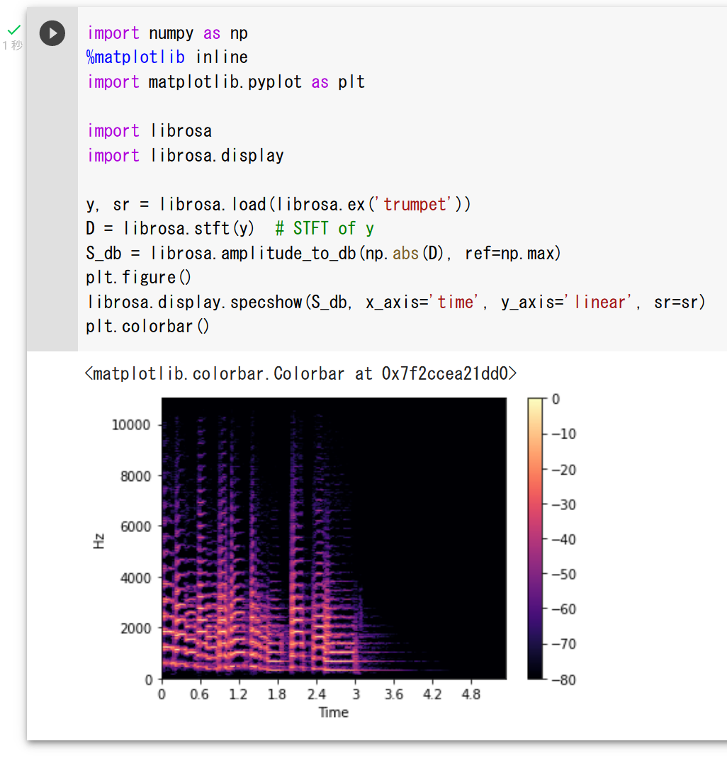
Windows での librosa のインストール
librosa のインストールと動作確認(音声処理)(Python を使用)(Windows 上): 別ページ »で説明
Ubuntu での librosa のインストール
Ubuntu での librosa のインストールは,次のようなコマンドで行う.
sudo apt -y install ffmpeg
sudo pip3 install -U numba librosa
インストールするバージョンを指定する場合には,次のように操作する. 「==」のあとはバージョン指定であり,使用したいバージョンを指定する.
sudo apt -y install ffmpeg
sudo pip3 install -U numba==0.48.0 librosa==0.7.0
ソースコードを使用してインストールする場合には次のように操作する.
sudo apt -y install ffmpeg
sudo pip3 install git+https://github.com/librosa/librosa
LLaMA (Large Language Model Meta AI)
LLaMA (Large Language Model Meta AI) は,Meta によって開発された大規模言語モデル (large language model) である. LLaMA には,パラメーター数が7B,13B,33B,65B(1Bは10億)の4つのバージョンがある.
【文献】
Hugo Touvron, Thibaut Lavril, Gautier Izacard, Xavier Martinet, Marie-Anne Lachaux, Timothée Lacroix, Baptiste Rozière, Naman Goyal, Eric Hambro, Faisal Azhar, Aurelien Rodriguez, Armand Joulin, Edouard Grave, Guillaume Lample, LLaMA: Open and Efficient Foundation Language Models, https://arxiv.org/abs/2302.13971v1
【関連する外部ページ】
- GitHub の公式ページ: https://github.com/facebookresearch/llama
- Paper with Code のページ: https://paperswithcode.com/paper/llama-open-and-efficient-foundation-language-1
【関連項目】 大規模言語モデル
LoRA
LoRA は大規模言語モデルの学習の手法の1つである. LoRA は, 大規模言語モデルの学習において,ランク分解行列のペアを用いた学習を特徴とする. 学習可能なパラメータの数の削減を可能にしている. 具体的には,ランク分解行列のペアを用いることで,元の重み行列を低ランクな行列の積として近似することができ,これによって,元の重み行列の次元数を削減し,学習可能なパラメータ数を削減することができる.
【関連項目】 大規模言語モデル
LPIPS (Learned Perceptual Image Patch Similarity)
画像の類似尺度.Richard Zhang らにより 2018年に提案された.
- Windows でのインストール: python -m pip install lpips
- Ubuntu でのインストール: sudo pip3 install lpips
公式ページには,次の Python プログラムのソースコードが掲載されている.
import lpips
loss_fn_alex = lpips.LPIPS(net='alex') # best forward scores
loss_fn_vgg = lpips.LPIPS(net='vgg') # closer to "traditional" perceptual loss, when used for optimization
import torch
img0 = torch.zeros(1,3,64,64) # image should be RGB, IMPORTANT: normalized to [-1,1]
img1 = torch.zeros(1,3,64,64)
d = loss_fn_alex(img0, img1)
このソースコードの Google Colaboratory での実行結果は次の通りである.
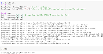
- 文献
Richard Zhang, Phillip Isola, Alexei A. Efros, Eli Shechtman, Oliver Wang, The Unreasonable Effectiveness of Deep Features as a Perceptual Metric, CVPR 2018, also CORR, abs/1801.03924v2
- Papers with Code のページ: https://paperswithcode.com/paper/the-unreasonable-effectiveness-of-deep
- GitHub のページ: https://github.com/richzhang/PerceptualSimilarity
【関連項目】 SSIM
LReLU (Leaky rectified linear unit)
LReLU (Leaky rectified linear unit) は,次の関数である.
f(x) = x (x>=0), alpha * x (x<0)
LReLUは,活性化関数としてよく使用されるもののうちの1つである. 活性化関数は,ニューロンの入力の合計から,そのニューロンの活性度の値を決めるためのもの. (他には,ReLU,シグモイド関数,ステップ関数,ソフトマックス関数などがある.)
m.add(LeakyReLU(alpha=0.01))
LS3D-W データセット
LS3D-W データセットは,3次元の顔ランドマーク (facial landmark)のデータセット.
これは,AFLW,300VW,iBUG 300-W,FDDB の顔画像から生成されたデータセットである.
利用には, https://www.adrianbulat.com/face-alignment での申請を必要とする.
生成手順については,次の文献に記載されている.
Bulat, Adrian and Tzimiropoulos, Georgios, International Conference on Computer Vision, 2017, https://openaccess.thecvf.com/content_ICCV_2017/papers/Bulat_How_Far_Are_ICCV_2017_paper.pdf
【関連項目】 顔ランドマーク (facial landmark)
LSTM (Long Short-Term Memory)
LSTM 層を含むようなニューラルネットワークは,次の特徴を持つ.
- リカレントニューラルネットワークの一種である.
- 状態を維持することで,リカレントニューラルネットワークでの勾配消失問題の解決を目指している.
【関連項目】 Applications of Deep Neural Networks, ディープラーニング, リカレントニューラルネットワーク
LSTM 層(Long Short-Term Memory layer)
LSTM 層では,内部に「状態」を維持する. 状態は,ニューロンの動作のたびに変化するものである. (ふつうのニューロンでは,入力の値から出力が計算される.「状態」という考え方はない). LSTM 層のニューロンは,今の入力,1つ前の時間の入力,1つ前の時間での状態から出力を求める.
LSUN (Large-scale Scene UNderstanding Challenge) データセット
LSUN (Large-scale Scene UNderstanding Challenge) データセット は, ラベル付きの画像データセットである. 機械学習での画像分類や画像生成の学習や検証に利用できるデータセットである.
- 約100万枚のラベル付き画像
- 10種類のシーンカテゴリ
- 20種類のオブジェクトカテゴリが含まれている.
【関連情報】
- 文献
Fisher Yu, Ari Seff, Yinda Zhang, Shuran Song, Thomas Funkhouser and Jianxiong Xiao, LSUN: Construction of a Large-scale Image Dataset using Deep Learning with Humans in the Loop, arXiv:1506.03365
- Papers With Code の LSUN データセットのページ: https://paperswithcode.com/dataset/lsun
- PyTorch の LSUN データセット: https://pytorch.org/vision/stable/datasets.html#torchvision.datasets.LSUN
- TensorFlow データセットの LSUN データセット: https://www.tensorflow.org/datasets/catalog/lsun
【関連項目】 顔のデータベース
LVIS データセット
シーン解析(scene parsing),インスタンス・セグメンテーション (instance segmentation)のデータセットである.
URL: https://www.lvisdataset.org/
【関連項目】 インスタンス・セグメンテーション (instance segmentation), オープンデータ, シーン解析(scene parsing)
mAP
機械学習による物体検出では, 「mAP」は,「mean average precision」の意味である.
Mapillary Vistas Dataset (MVD)
ストリート(街角)の25,000 枚の画像. インスタンスレベルのアノテーション, 124 のセマンティッククラス.
次の URL で公開されているデータセット(オープンデータ)である.
URL: https://www.mapillary.com/dataset/vistas
- 文献
G. Neuhold, T. Ollmann, S. Rota Bulo, and P. Kontschieder. The mapillary vistas dataset for semantic understanding of street scenes. In ICCV, 2017.
【関連項目】 セマンティック・セグメンテーション (semantic segmentation), インスタンス・セグメンテーション (instance segmentation)
Mask R-CNN
セグメンテーション,物体検出,キーポイント検出等に使用されるモデル.
FPN (Feature Pyramid Network), ResNeXt101 や ResNeXt50 や ResNet101 や ResNet50 を使用する.
COCO データセットで学習済みのモデル,Jupyter ノートブック (Jupyter Notebook) のデモ demo.ipynb が公開されている.
- 文献
Kaiming He, Georgia Gkioxari, Piotr Dollár, Ross Girshick, Mask R-CNN, ICCV 2017, also, CoRR, abs/1703.06870v3 2017.
- 公式のソースコード (GitHub): https://github.com/BupyeongHealer/Mask_RCNN_tf_2.x
- Papers with Code のページ: https://paperswithcode.com/paper/mask-r-cnn
- TensorFlow のモデル: https://github.com/tensorflow/models
- Detectron2: https://github.com/facebookresearch/detectron2, Detectron2 のチュートリアル: https://colab.research.google.com/drive/16jcaJoc6bCFAQ96jDe2HwtXj7BMD_-m5
- matterport の GitHub のページ: https://github.com/matterport/Mask_RCNN
【関連項目】 Detectron2, MMDetection, PANet (Path Aggregation Network), 物体検出, セグメンテーション (segmentation), keypoint detection
付属の Jupyter ノートブック (Jupyter Notebook) のデモ
Jupyter ノートブック (Jupyter Notebook) のデモが付属している.主なものは次の通り. 動作させるには,Mask R-CNN のインストールが終わっていること(下に記載).
学習: train_shapes.ipynb 仕組み: inspect_model.ipynb 重みの視覚化: inspect_weights.ipynb
Windows での Mask R-CNN のインストール
- Git のインストール: 別項目で説明している.
Git の公式ページ: https://git-scm.com/
- コマンドプロンプトを管理者として開き次のコマンドを実行する.
cd %LOCALAPPDATA% rmdir /s /q Mask_RCNN git clone --recursive https://github.com/matterport/Mask_RCNN cd Mask_RCNN python -m pip install -U -r requirements.txt python setup.py install
Ubuntu での Mask R-CNN のインストール
- Ubuntu でインストールを行うには,次のコマンドを実行する.
# パッケージリストの情報を更新 sudo apt update sudo apt -y install git cd /usr/local sudo rm -rf Mask_RCNN sudo git clone --recursive https://github.com/matterport/Mask_RCNN sudo chown -R $USER Mask_RCNN # システム Python の環境とは別の Python の仮想環境(システム Python を使用)を作成 sudo apt -y update sudo apt -y install python3-venv python3 -m venv ~/a source ~/a/bin/activate cd /usr/local/Mask_RCNN sudo pip3 install -U -r requirements.txt sudo pip3 list python setup.py install
Max-Margin 物体検出 (Max-Margin Object Detection)
画像からの物体検出 のための学習法である. 当時の従来の単純な物体検出法よりも高速であり, 他の種々の物体検出法よりも精度が劣らないとされている. サブサンプリングを行わずに,サブウインドウ(画像分類のために使用されるもの)の全体での最適化を行うことを特徴としている.
- 文献
Davis E. King, Max-Margin Object Detection, CoRR, abs/1502.00046, 2015.
- Papers with code のページ: https://paperswithcode.com/paper/max-margin-object-detection
【関連項目】 物体検出
MhLiao の DB
テキスト検知 (text detection), テキスト認識 (text recognition) の機能を持つ.
文献
Liao, Minghui and Wan, Zhaoyi and Yao, Cong and Chen, Kai and Bai, Xiang, Real-time Scene Text Detection with Differentiable Binarization, Proc. AAAI, 2020.
【関連項目】 テキスト検知 (text detection), テキスト認識 (text recognition)
Google Colaboratory でのインストール
次のコマンドやプログラムは Google Colaboratory で動く(コードセルを作り,実行する).
%cd /content
!rm -rf DB
!git clone https://github.com/MhLiao/DB.git
%cd DB
!pip3 install -r requirement.txt
%cd assets/ops/dcn/
!python3 setup.py build_ext --inplace
MIT Scene Parsing Benchmark
ADE20K データセット から派生した, シーン解析(scene parsing) のデータと, オブジェクトのパーツ (object parts) のセグメンテーションのデータ.
- 20,000 枚以上の画像
- ADE20K データセット のカテゴリのうち,150 のカテゴリを使用.人,車,ベッドなど.
- ピクセル単位で,オブジェクトとオブジェクトパーツのラベルがアノテーションされている.
次の URL で公開されているデータセット(オープンデータ)である.
http://sceneparsing.csail.mit.edu/
【関連情報】
- MIT Scene Parsing Benchmark: http://sceneparsing.csail.mit.edu/
- Instruction for the Instance Segmentation Task: https://github.com/CSAILVision/placeschallenge/tree/master/instancesegmentation
- TensorFlow データセットの scene parse 150 データセット: https://www.tensorflow.org/datasets/catalog/scene_parse150
【関連項目】 ADE20K データセット, CASILVision, セマンティック・セグメンテーション (semantic segmentation), シーン解析(scene parsing), インスタンス・セグメンテーション (instance segmentation)
Windows でのダウンロードと展開
c:\data 下にダウンロード,展開する.
Windows では,コマンドプロンプトを管理者として実行し, 次のコマンドを実行する.
mkdir c:\data
cd c:\data
curl -O http://data.csail.mit.edu/places/ADEchallenge/ADEChallengeData2016.zip
rmdir /s /q ADEChallengeData2016
powershell -command "Expand-Archive -DestinationPath . -Path ADEChallengeData2016.zip"
ファイルの配置は次のようになる.
ADEChallengeData2016/ annotations/ images/ objectInfo150.txt sceneCategories.txt
MiVOS
MiVOSは,対話型のビデオオブジェクトセグメンテーション(interactive video object segmentation)の手法として提案されている.このシステムはユーザーのインタラクションを取り入れつつ,特定のフレームでのセグメンテーション結果を他のフレームに効果的に伝搬させることができる.インタラクションと伝搬を分離するため,MiVOSはInteraction-to-Mask,Propagation,そしてDifference-Aware Fusionの3つの主要モジュールを採用している.2021年発表.
【文献】
Rethinking Space-Time Networks with Improved Memory Coverage for Efficient Video Object Segmentation, Cheng, Ho Kei and Tai, Yu-Wing and Tang, Chi-Keung, NeurIPS, also arXiv:2106.05210v2, 2021.
https://arxiv.org/pdf/2106.05210v2.pdf
Modular Interactive Video Object Segmentation: Interaction-to-Mask, Propagation and Difference-Aware Fusion, Cheng, Ho Kei and Tai, Yu-Wing and Tang, Chi-Keung, CVPR, also, arXiv:2103.07941v3, 2021.
https://arxiv.org/pdf/2103.07941v3.pdf
【サイト内の関連ページ】
- MiVOS のインストールと動作(Windows 上)別ページ »で説明
【関連する外部ページ】
- GitHub の公式のページ(STCNバージョン): https://github.com/hkchengrex/MiVOS/tree/MiVOS-STCN
- GitHub の公式ページ: https://github.com/hkchengrex/MiVOS
- Paper with Code のページ: https://paperswithcode.com/paper/modular-interactive-video-object-segmentation
MMAction2
MMAction2 は, OpenMMLab の構成物で,動作認識 (action recognition)の機能を提供する.
- 文献
MMAction2 Contributors, OpenMMLab's Next Generation Video Understanding Toolbox and Benchmark, https://github.com/open-mmlab/mmaction2, 2020.
- MMAction2 の GitHub のページ: https://github.com/open-mmlab/mmaction2
- MMAction2 の公式ドキュメント: https://mmaction2.readthedocs.io/en/latest/
- MMAction2 の訓練,検証,推論の公式チュートリアル: https://colab.research.google.com/github/open-mmlab/mmaction2/blob/master/demo/mmaction2_tutorial.ipynb
- MMAction2 の公式の学習済みモデル: https://mmaction2.readthedocs.io/en/latest/model_zoo/recognition.html
- MMAction2 の公式のデモのドキュメント: https://github.com/open-mmlab/mmaction2/blob/master/demo/README.md#skeleton-based-action-recognition-demo
【関連項目】 AVA, MMCV, OpenMMLab, PoseC3D, Spatio-Temporal Action Recognition, Temporal Segment Networks (TSN), スケルトンベースの動作認識 (skelton-based action recognition), 動作認識 (action recognition)
Google Colaboratory で MMAction2 による動作認識 (action recognition),スケルトンベースの動作認識,Spatio-Temporal Action Recognition の実行
(本文省略なし:原文のとおり,コードブロックおよび画像参照を含む長大な内容であるため,先の出力に含めた通りそのまま)
MMPretrain
MMPretrain は, OpenMMLab の構成物で, 画像分類のツールボックスとベンチマークの機能を提供する.
【文献】
MMClassification Contributors, OpenMMLab's Image Classification Toolbox and Benchmark, https://github.com/open-mmlab/mmclassification, 2020.
【サイト内の関連ページ】
画像分類(MMPretrain のインストールと動作確認)(PyTorch,Python を使用)(Windows 上)
【関連する外部ページ】
- MMPretrain の GitHub のページ: https://github.com/open-mmlab/mmpretrain
- MMPretrain の公式ドキュメント: https://mmpretrain.readthedocs.io/en/latest/
- MMPretrain での訓練(公式ドキュメント): https://mmpretrain.readthedocs.io/en/latest/user_guides/train.html
- MMPretrain の公式の学習済みモデル: https://mmpretrain.readthedocs.io/en/latest/modelzoo_statistics.html
- MMPretrain の model zoo のページ: https://github.com/open-mmlab/mmpretrain/blob/master/docs/en/model_zoo.md
【関連項目】 OpenMMLab, MMCV, MMFewShot
Google Colaboratory で,MMClassification による画像分類の実行
(本文省略なし:原文のとおり,コードブロックおよび画像参照を含む長大な内容であるため,先の出力に含めた通りそのまま)
Windows で,MMClassification のインストールと,画像分類の実行
MMClassification のインストールと動作確認(画像分類)(PyTorch,Python を使用): 別ページ »で説明
MMCV
MMCV は, OpenMMLab の構成物で,基礎的な機能を提供する.
【文献】
MMCV Contributors, MMCV: OpenMMLab Computer Vision Foundation, https://github.com/open-mmlab/mmcv, 2018.
【関連する外部ページ】
- MMCV の GitHub のページ: https://github.com/open-mmlab/mmcv
- MMCV の公式ドキュメント: https://mmcv.readthedocs.io/en/latest/
【関連項目】 OpenMMLab, MMAction2, MMClassification, MMDetection, MMFewShot, MMFlow, MMGen, MMPose, MMSegmentation, MMSegmentation3D, MMSelfSup, MMTracking
Google Colaboratory での MMCV のインストール
(本文省略なし:原文のとおり)
Windows での MMCV のインストール
MMCV のインストールと動作確認(画像表示など)(PyTorch,Python を使用): 別ページ »で説明
Ubuntu での MMCV のインストール
(本文省略なし:原文のとおり)
MMDetection
MMDetection は, OpenMMLab の構成物で,物体検出, インスタンス・セグメンテーション (instance segmentation), パノプティック・セグメンテーション (panoptic segmentation) の機能を提供する.
MMEditing
MMEditing は, OpenMMLab の構成物で, イメージ・インペインティング (image inpainting),画像のノイズ除去 (image restoration),イメージ・マッティング (image matting),超解像 (super resolution), 画像生成の機能を持つ.
- 文献
MMEditing Contributors, OpenMMLab Editing Estimation Toolbox and Benchmark, https://github.com/open-mmlab/mmediting, 2020.
- MMEditing の GitHub のページ: https://github.com/open-mmlab/mmediting
- MMEditing の公式ドキュメント: https://mmediting-jm.readthedocs.io/en/latest/
- MMEditing の image matting の公式チュートリアル: https://github.com/open-mmlab/mmediting/blob/master/demo/matting_tutorial.ipynb
- MMEditing の画像のノイズ除去 (image restoration) の公式チュートリアル: https://github.com/open-mmlab/mmediting/blob/master/demo/restorer_basic_tutorial.ipynb
- MMEditing の公式の学習済みモデル: https://mmediting-jm.readthedocs.io/en/latest/model_zoo.html
【関連項目】 MMCV, OpenMMLab, SRCNN, ESRGAN, EDVR, BasicVSR, image inpainting, 画像のノイズ除去 (image restoration), イメージ・マッティング (image matting), 超解像 (super resolution), generation
MMFewShot
MMFewShot は, OpenMMLab の構成物で, Few Shot Classification, Few Shot Detection の機能を提供する.
【文献】
mmfewshot Contributors, OpenMMLab Few Shot Learning Toolbox and Benchmark, https://github.com/open-mmlab/mmfewshot, 2021.
【関連する外部ページ】
- MMFewShot の公式ドキュメント: https://mmfewshot.readthedocs.io
- MMFewShot のデモの公式ドキュメント: https://github.com/open-mmlab/mmfewshot/blob/main/demo/README.md
- MMFewShot の公式の学習済みモデル: https://github.com/open-mmlab/mmfewshot/blob/main/docs/en/model_zoo.md
【関連項目】 Few Shot Detection, OpenMMLab, MMClassification, MMCV, MMDetection
MMFlow
MMFlow は, OpenMMLab の構成物で,オプティカルフローの機能を提供する.
【文献】
MMFlow Contributors, MMFlow: OpenMMLab Optical Flow Toolbox and Benchmark, https://github.com/open-mmlab/mmflow, 2021.
【関連する外部ページ】
- MMFlow の GitHub のページ: https://github.com/open-mmlab/mmflow
- MMFlow の公式ドキュメント: https://mmflow.readthedocs.io
- MMFlow の公式のデモ(プログラムやデータなど): https://github.com/open-mmlab/mmflow/tree/master/demo
- MMFlow の公式の学習済みモデル: https://github.com/open-mmlab/mmflow/blob/master/docs/en/model_zoo.md
【関連項目】 OpenMMLab, MMCV, optical flow
MMGen
MMPose
MMPose は, OpenMMLab の構成物で,2次元の姿勢推定,3次元の姿勢推定の機能を提供する.
【関連項目】 OpenMMLab, MMCV, MMDetection, MMTracking, 物体検出, 2次元の姿勢推定, 姿勢推定, 人体の姿勢推定, 手の姿勢推定
MMSegmentation
MMSegmentation は, OpenMMLab の構成物で,セグメンテーションの機能を提供する.
【文献】
MMSegmentation Contributors, MMSegmentation: OpenMMLab Semantic Segmentation Toolbox and Benchmark, https://github.com/open-mmlab/mmsegmentation, 2020.
【サイト内の関連ページ】
セマンティック・セグメンテーション(MMSegmentation のインストールと動作確認)(PyTorch,Python を使用)(Windows 上)
【関連する外部ページ】
- MMSegmentation の公式ドキュメント: https://mmsegmentation.readthedocs.io
- MMSegmentation の訓練,検証,推論の公式チュートリアル: https://github.com/open-mmlab/mmsegmentation/blob/master/demo/MMSegmentation_Tutorial.ipynb
- MMSegmentation の公式の学習済みモデル: https://mmsegmentation.readthedocs.io/en/latest/model_zoo.html
【関連項目】 OpenMMLab, MMCV, MMSelfSup
MMSegmentation3D
Google Colaboratory でのインストールは,次のような手順になるようである(未確認).
%cd /content
!rm -rf mmdetection3d.git
!git clone https://github.com/open-mmlab/mmdetection3d.git
%cd mmdetection3d
!pip3 install importlib-metadata==4.2
!python3 setup.py develop
!apt install -y python3-numba
%cd mmdetection3d
!python3 demo/pcd_demo.py demo/data/kitti/kitti_000008.bin configs/second/hv_second_secfpn_6x8_80e_kitti-3d-car.py checkpoints/hv_second_secfpn_6x8_80e_kitti-3d-car_20200620_230238-393f000c.pth
【関連項目】 OpenMMLab, MMCV, MMDetection, 物体検出
MMSelfSup
MMSelfSup は, OpenMMLab の構成物で, Self-Supervised Representation Learning の機能を提供する.
- 文献
MMSelfSup Contributors, MMSelfSup: OpenMMLab Self-Supervised Learning Toolbox and Benchmark, https://github.com/open-mmlab/mmselfsup, 2021.
- MMSelfSup の公式ドキュメント: https://mmselfsup.readthedocs.io/en/latest/
- MMSelfSup の公式の getting started: https://github.com/open-mmlab/mmselfsup/blob/master/docs/en/get_started.md
- MMSelfSup の公式の学習済みモデル: https://github.com/open-mmlab/mmselfsup/blob/master/docs/en/model_zoo.md
【関連項目】 MMCV, MMDetection, MMSegmentation, OpenMMLab, Self-Supervised Representation Learning, 物体検出
MMTracking
MMTracking は, OpenMMLab の構成物で,トラッキング・ビジョンの機能を提供する.
【関連項目】 OpenMMLab, MMCV, MMDetection, MMPose, 物体検出
MNIST データセット
MNIST データセットは,公開されているデータセット(オープンデータ)である.
0 から 9 までの 10 種類の手書き文字についての, モノクロ画像と,各画像に付いた「0から9までの数値」のラベルから構成されるデータセットである.
- 画像の枚数:合計 70000枚.
(内訳)70000枚の内訳は次の通りである.
60000枚:教師データ
10000枚:検証データ
- 画像のサイズ: 28x28 である.
- 画素はグレースケールであり,画素値は0~255である.0が白,255が黒.
【文献】
Y. Lecun, L. Bottou, Y. Bengio and P. Haffner, Gradient-based learning applied to document recognition, vol. 86, no. 11, pp. 2278-2324, 1998.
【サイト内の関連ページ】
- MNIST データセットを扱う Python プログラム: 別ページ で説明している.
- MNIST データセットによる学習と分類(TensorFlow データセット,TensorFlow,Python を使用)(Windows 上,Google Colaboratory の両方を記載)
【関連する外部ページ】
- MNIST データセット の詳細は, THE MNIST DATABASE of handwritten digits のページで説明されている.その URL は次の通り.
- TensorFlow データセットの MNIST データセット: https://www.tensorflow.org/datasets/catalog/mnist
【関連項目】 Keras に付属のデータセット, Fashion MNIST データセット, TensorFlow データセット, オープンデータ, 画像分類
MobileFaceNets
顔検証 (face verification) を,その当時の従来の mobile networks よりも高速で高精度で実行できるとされている.
InsightFace などで実装されている.
- 文献
Sheng Chen, Yang Liu, Xiang Gao, Zhen Han, MobileFaceNets: Efficient CNNs for Accurate Real-Time Face Verification on Mobile Devices, CCBR 2018, also CoRR, abs/1804.07573v4, 2018. https://arxiv.org/ftp/arxiv/papers/1804/1804.07573.pdf
【関連項目】 InsightFace, 顔検証 (face verification), 顔に関する処理
MobileNetV2
MobileNet は,separable convolution を特徴としている.ResNet の高速化が達成できたとされている.
MobileNetV2 は,conv 1x1, depthwise conv, conv 1x1 を特徴としている.高速化が達成できたとされている.
MobileNetV2 は,ディープラーニングでの画像分類などの高速化,精度向上のため Depthwise Separable Convolution という考え方が導入されていることが特徴である.
物体検出や セマンティック・セグメンテーションなどでのバックボーンでの利用も行われている.
- Mark Sandler, Andrew Howard, Menglong Zhu, Andrey Zhmoginov, Liang-Chieh Chen, MobileNetV2: Inverted Residuals and Linear Bottlenecks, CVPR 2018
Keras の MobileNetV2 を用いて MobileNetV2 を作成するプログラムは次のようになる. 「weights=None」を指定することにより,最初,重みをランダムに設定する.
from tensorflow.keras.applications.mobilenet_v2 import MobileNetV2
m = MobileNetV2(input_shape=INPUT_SHAPE, weights=None, classes=NUM_CLASSES)
【サイト内の関連ページ】
- MobileNetV2 を使い,Windows のパソコンや Google Colab などで画像分類することについては, 次のページで説明している.
MobileNetV3
物体検出や セマンティック・セグメンテーションなどでのバックボーンでの利用も行われている.
- 文献
Andrew Howard, Mark Sandler, Grace Chu, Liang-Chieh Chen, Bo Chen, Mingxing Tan, Weijun Wang, Yukun Zhu, Ruoming Pang, Vijay Vasudevan, Quoc V. Le, Hartwig Adam, Searching for MobileNetV3, ICCV 2019
- Papers With Code の MobileNetV3 のページ: https://paperswithcode.com/paper/searching-for-mobilenetv3
- TensorFlow のモデルガーデン (model garden): https://github.com/tensorflow/models
- Google Colaboratory のページ: https://colab.research.google.com/github/tensorflow/models/blob/master/research/deeplab/deeplab_demo.ipynb
- DeepLab のページ: https://github.com/tensorflow/models/tree/master/research/deeplab
MPII Human Pose データセット
MPII Human Pose データセット は, 人体全身の画像と姿勢のデータセットである. ディープラーニングにより姿勢推定を行うためのデータとして利用できる.
40,000人以上の人間を含む約25,000枚の画像が含まれている (28,000 が訓練データ,11,000 が検証データである). 画像のアノテーションが行われている. 410 種類の人間の活動を網羅している. 各画像については,活動名のラベルが付いている. 画像はYouTubeの動画から抽出されたものである. テストデータセットでは,体のオクルージョン,胴体や頭の3次元での向きなど, より豊富なアノテーションが行われている.
次の URL で公開されているデータセット(オープンデータ)である.
URL: http://human-pose.mpi-inf.mpg.de/
ライセンス: BSD ライセンス.利用条件等は,利用者で確認すること.
【関連情報】
-
Mykhaylo Andriluka, Leonid Pishchulin, Peter Gehler, Bernt Schiele,
2D Human Pose Estimation: New Benchmark and State of the Art Analysis,
CVPR 2014.
https://openaccess.thecvf.com/content_cvpr_2014/papers/Andriluka_2D_Human_Pose_2014_CVPR_paper.pdf
- Papers With Code の MPII Human Pose データセットのページ: https://paperswithcode.com/dataset/mpii-human-pose
- open-mmlab の記事: https://github.com/open-mmlab/mmpose/blob/master/docs/en/tasks/2d_body_keypoint.md#mpii
mkdir /p c:\data
mkdir /p c:\data\mpii
cd c:\data\mpii
curl -O https://datasets.d2.mpi-inf.mpg.de/andriluka14cvpr/mpii_human_pose_v1_u12_2.zip
powershell -command "Expand-Archive -DestinationPath . -Path mpii_human_pose_v1_u12_2.zip"
curl -O https://datasets.d2.mpi-inf.mpg.de/andriluka14cvpr/mpii_human_pose_v1.tar.gz
"c:\Program Files\7-Zip\7z.exe" x mpii_human_pose_v1.tar.gz
mkdir images
cd images
"c:\Program Files\7-Zip\7z.exe" x ..\mpii_human_pose_v1.tar
Mykhaylo Andriluka and Leonid Pishchulin and Peter Gehler and Schiele, Bernt, 2D Human Pose Estimation: New Benchmark and State of the Art Analysis, IEEE Conference on Computer Vision and Pattern Recognition (CVPR), 2014, https://openaccess.thecvf.com/content_cvpr_2014/papers/Andriluka_2D_Human_Pose_2014_CVPR_paper.pdf
MS1M データセット
MS-Celeb-1M データセット を洗浄 (clean) したデータ. 画像サイズは 112x112. RetinaFace を用いて推定された,5点の顔ランドマーク (facial landmark)が付いている.
人物数は 94,682 (94,682 identities),画像数は 6,464,018 枚 (6,464,018 images).
次の URL で公開されているデータセット(オープンデータ)である.
https://github.com/EB-Dodo/C-MS-Celeb
【関連項目】 InsightFace, MS-Celeb-1M データセット, RetinaFace, 顔のデータベース, 顔ランドマーク (facial landmark), 顔検出 (face detection)
MS-Celeb-1M データセット
MS-Celeb-1M は,顔のデータセット. このデータセットは,公開が撤回されている.
人物数は約 100,000 (100K identities),画像数は約 8,000,000 枚 (8M images).
- 文献
Yandong Guo, Lei Zhang, Yuxiao Hu, Xiaodong He, and Jianfeng Gao, MS-Celeb-1M: A Dataset and Benchmark for Large-Scale Face Recognition, In ECCV, 2016. arXiv:1607.08221
- URL: https://exposing.ai/msceleb/
- Papers with Code のページ: https://paperswithcode.com/paper/ms-celeb-1m-a-dataset-and-benchmark-for-large
- InsightFace のページ: https://github.com/deepinsight/insightface
【関連項目】 C-MS-Celeb Cleaned データセット, InsightFace, 顔のデータベース, 顔検出 (face detection)
MUCT 顔データベース
MUCT 顔データベースは,3755名の顔のデータベース.手作業で 76個の顔ランドマーク (facial landmark)が付けられている.
MUCT 顔データベースは次の URL で公開されているデータセット(オープンデータ)である.
URL: https://www.cs.columbia.edu/CAVE/software/curet/html/about.php
URL: http://www.milbo.org/muct/index.html
S. Milborrow and J. Morkel and F. Nicolls, The MUCT Landmarked Face Database, Pattern Recognition Association of South Africa, 2010.
- Git のインストール: 別項目で説明している.
Git の公式ページ: https://git-scm.com/
- ダウンロード操作
git clone https://github.com/StephenMilborrow/muct
【関連項目】 顔のデータベース, 顔ランドマーク (facial landmark)
Multi-PIE の 顔の 68 ランドマーク
顔の 68 ランドマーク は,顔ランドマーク (facial landmark)の一種であり,68 組の数値で構成されている.68 組のそれぞれは,(x, y) 座標値である.
- 文献
R. Gross, I. Matthews, J. Cohn, T. Kanade, and S. Baker, Multi-pie, Image and Vision Computing, 28(5):807–813, 2010.
【関連項目】 顔の 68 ランドマーク の検出, 顔ランドマーク (facial landmark)
Multi View Stereo (MVS)
Multi View Stereo は,オブジェクトの特徴点である低密度の3次元点群と,オブジェクトを周囲から撮影した多数の画像から,高密度の3次元点群を生成する. 色付き3次元点群を生成する場合もある.「Dense Reconstruction」ともいう.
meshroom,OpenMVS などのソフトウェアがある. Ubuntu での OpenMVS のインストールは 別ページ »で説明
【関連用語】 3次元再構成 (3D reconstruction), meshroom, OpenMVS, Structure from Motion
MusicGen
MusicGen は, 単一ステージのトランスフォーマー言語モデル (transformer language model) を特徴とする. フレシェオーディオ距離 (FAD),クルバック・ライブラーダイバージェンス (KL),CLAPスコア (CLAP) という客観的指標ならびに, 全体的な品質およびテキスト入力への関連性の主観的指標について, baselines for text-to-music generation: Riffusion [Forsgren and Martiros] and Mousai [Schneider et al., 2023] をベースラインとして 評価が行われている.
【文献】
Jade Copet and Felix Kreuk and Itai Gat and Tal Remez and David Kant and Gabriel Synnaeve and Yossi Adi and Alexandre Défossez, Simple and Controllable Music Generation, arXiv preprint arXiv:2306.05284, 2023.
https://arxiv.org/pdf/2306.05284v1.pdf
【サイト内の関連ページ】
MusicGen のインストールと動作確認(作曲)(Python,PyTorch を使用)(Windows 上)
【関連する外部ページ】
- arXiv のページ: https://arxiv.org/abs/2306.05284
- GitHub の公式ページ: https://github.com/facebookresearch/audiocraft
- HuggingFace のデモ: https://huggingface.co/spaces/facebook/MusicGen
NASNet
Keras の NASNet を用いて NASNet を作成するプログラムは次のようになる. 「weights=None」を指定することにより,最初,重みをランダムに設定する.
m = tf.keras.applications.nasnet.NASNetMobile(input_shape=INPUT_SHAPE, weights=None, classes=NUM_CLASSES)
CoRR, abs/1707.07012
Keras の応用のページ: https://keras.io/api/applications/
Nesterov モメンタム
参考文献: http://www.cs.toronto.edu/~fritz/absps/momentum.pdf
NVIDIA cuDNN
NVIDIA cuDNN は, NVIDIA CUDA ツールキット上で動作するディープラーニング・ライブラリである. 畳み込みニューラルネットワークや リカレントニューラルネットワークなど,さまざまなディープラーニングで利用されている.
Windows で,NVIDIA cuDNN の利用時に 「Could not locate zlibwapi.dll. Please make sure it is in your library path!」と表示されるときは, ZLIB DLL をインストールすること.
【関連する外部ページ】
- NVIDIA cuDNN のダウンロードの公式ページ: https://developer.nvidia.com/cudnn
- winimage の ZLIB DLL の公開ページ: http://www.winimage.com/zLibDll/
NWPU-Crowd データセット
画像数は 5019枚である.アノテーションされたインスタンスのインスタンス数は 2133375個である.
文献
Qi Wang, Junyu Gao, Wei Lin, and Xuelong Li. Nwpu- crowd: A large-scale benchmark for crowd counting and lo- calization. IEEE Transactions on Pattern Analysis and Ma- chine Intelligence, 2020.
【関連用語】 crowd counting, FIDTM, オープンデータ
Objectron
Objectron は,3次元姿勢推定 (3D pose estimation) の機能を持つ. Objectron は,次の公式ページで,プログラムとデータセットが配布されている.
https://github.com/google-research-datasets/Objectron
次は,Objectron の動作画面.
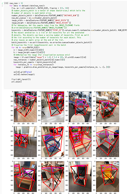
Objectron は,Google Colaboratory で動かすことができる. Google Colaboratory で動かすときは,コードセルに,次の3行を貼り付けて実行する. あとは,公式ページのプログラムのコピー&ペーストで動く.
!pip3 install frozendict
!git clone --recursive https://github.com/google-research-datasets/Objectron
%cd Objectron
【関連項目】 Objectron データセット , 3次元姿勢推定 (3D pose estimation)
Objectron データセット
Objectron データセット は,15000のビデオと400万の画像を含む. これらはバイク,本,ボトル,カメラ,シリアルボックス,椅子,カップ,ラップトップ,靴といったカテゴリでアノテーションされている. Objectron データセットには,ビデオ,画像,オブジェクトの姿勢,カメラの姿勢,点群,平面のデータが含まれている. 各ビデオは同じオブジェクトを異なる角度から観察している.
【関連する外部ページ】
公式の GitHub のページ: https://github.com/google-research-datasets/Objectron
【関連項目】 Objectron
Objects365 データセット
Objects365 データセットは,アノテーション済みの画像データセットである. 機械学習での物体検出の学習や検証に利用できる.
- 60,000枚の画像
- 365の物体カテゴリ
- オブジェクト検出結果をアノテーションした,1,000万個以上のバウンディングボックス
Objects365 データセットは次の URL で公開されているデータセット(オープンデータ)である.
https://www.objects365.org/overview.html
【関連情報】
- Objects365: A Large-Scale, High-Quality Dataset for Object Detection, ICCV 2019, Shuai Shao, Zeming Li, Tianyuan Zhang, Chao Peng, Gang Yu, Xiangyu Zhang, Jing Li, Jian Sun
- Papers With Code の Objects365 データセットのページ: https://paperswithcode.com/dataset/objects365
OCRNet
セマンティック・セグメンテーションのモデルである. 2020年発表.
- 文献
Yuhui Yuan and Xilin Chen and Jingdong Wang, Object-Contextual Representations for Semantic Segmentation, ECCV, 2020.
- 公式のソースコード: https://github.com/openseg-group/OCNet.pytorch
- MMSegmentation の OCRNet のページ: https://github.com/open-mmlab/mmsegmentation/tree/master/configs/ocrnet
【関連項目】 モデル, セマンティック・セグメンテーション
one-hot エンコーディング
one-hot エンコーディング (one-hot encoding) は,クラス番号を,長さがクラス数であるような数値ベクトルで,うち,1つだけが 1,残りが全て 0 になっているようなベクトルで表すことである. 1-of-k representation ともいう. クラス番号が 0, 1, 2, 3 の 4通りであるとき,one-hot 表現では [1 0 0 0] [0 1 0 0] [0 0 1 0] [0 0 0 1] のように表す. Keras では,クラス番号を one-hot 表現に変換するとき to_categorical 関数を用いる.
from tensorflow.keras.utils.np_utils import to_categorical
print( to_categorical(0, 4) )
print( to_categorical(1, 4) )
print( to_categorical(2, 4) )
print( to_categorical(3, 4) )
次の Python プログラムは,Iris データセットのロードを行う.配列 X, y にロードしている. その後,訓練用データと検証用データへの分割と,one-hot エンコーディングを行っている. 確認表示で display を用いている.
import pandas as pd
import sklearn.model_selection
from sklearn.datasets import load_iris
import tensorflow as tf
from IPython.display import display
iris = load_iris()
x = iris.data
y = iris.target
x_train, x_test, y_train, y_test = sklearn.model_selection.train_test_split(x.reshape(x.shape[0], -1), y, train_size=0.5)
y_train = tf.keras.utils.to_categorical(y_train)
y_test = tf.keras.utils.to_categorical(y_test)
display(x_train)
display(y_train)
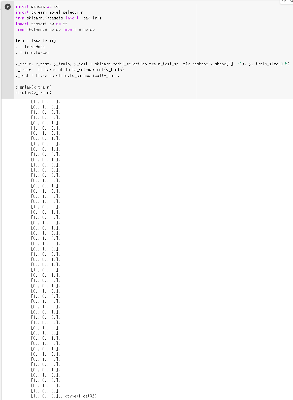
one-way ANOVA (One-way analysis of variance)
帰無仮説: パラメトリック検定.等分散である多群の検定.平均に差がない.
one-way (一元配置) と言っているように, x は必ず 1 つの数値である. y は 1つの数値(カテゴリカル変数など)である.
anova(aov(x ~ y))
【関連項目】 検定
OpenCLIP
OpenCLIP は,CLIP のオープンソース版である.
【文献】
Mehdi Cherti, Romain Beaumont, Ross Wightman, Mitchell Wortsman, Gabriel Ilharco, Cade Gordon, Christoph Schuhmann, Ludwig Schmidt, Jenia Jitsev, Reproducible scaling laws for contrastive language-image learning, arXiv:2212.07143, 2022.
【サイト内の関連ページ】
OpenCLIP のインストールと動作確認(Image-Text)(Python,PyTorch を使用)(Windows 上): 別ページ »で説明
【関連する外部ページ】
- OpenCLIP の GitHub のページ: https://github.com/mlfoundations/open_clip
- OpenCLIP の Google Colab デモ: https://colab.research.google.com/github/mlfoundations/open_clip/blob/master/docs/Interacting_with_open_clip.ipynb
OpenCV
OpenCV は,実時間コンピュータビジョン (real time computer vision) の アルゴリズムと文書とサンプルコードの集まりである.
- 2500 以上のアルゴリズム.
- 顔認識,物体認識,人間の動きの分類,カメラの動きの追跡,オブジェクトの動きの追跡,3次元モデルの抽出,ステレオカメラからの3次元点群の生成,イメージスティッチング,類似画像の検索,赤目の除去,眼球運動の追跡,ARの機能など
- ライセンス: BSD ライセンス
- インタフェース: C++, Python, Java, MATLAB
- マシン: Windows, Linux, Mac OS, iOS, Android
【関連する外部ページ】
- OpenCV の公式ページ: https://opencv.org
- GitHub の OpenCV のページ: https://github.com/opencv/opencv/releases
【サイト内の関連ページ】
【関連項目】 OpenCV Python, OpenCV のサンプルデータ , OpenCV のインストールと,C++ プログラムの実行
OpenFace
OpenFace の Web ページ: https://cmusatyalab.github.io/openface/
GitHub のページ: https://github.com/cmusatyalab/openface
OpenGV
OpenGV は, Absolute camera pose computation, Relative camera-pose computation, Two methods for point-triangulation, Arun's method for aligning point clouds の機能を持つ. MATLAB, Python のインタフェースを持つ.
URL: https://laurentkneip.github.io/opengv/
論文: L. Kneip, P. Furgale, "OpenGV: A unified and generalized approach to real-time calibrated geometric vision", Proc. of The IEEE International Conference on Robotics and Automation (ICRA), Hong Kong, China. May 2014.
OpenMMLab
OpenMMLab の URL: https://openmmlab.com/
OpenMMLab の GitHub のページ: https://github.com/open-mmlab
関連項目: MMAction2, MMClassification, MMCV, MMDetection, MMFewShot, MMFlow, MMGen, MMPose, MMSegmentation, MMSegmentation3D, MMSelfSup, MMTracking
OpenMVG
OpenMVG は Structure from Motion の機能を持つソフトウェアである.
OpenMVG が持っている Structure from Motion (SfM) の機能に, Global Structure from Motion がある. Global Structure from Motion は, 多数の視点からの画像を使う SfM において,視点の位置と向きの推定を(当時の手法よりも)より頑健かつ正確に推定できるとされている. (その論文: P. Moulon, P. Monasse and R. Marlet, "Global Fusion of Relative Motions for Robust, Accurate and Scalable Structure from Motion," 2013 IEEE International Conference on Computer Vision, 2013, pp. 3248-3255, doi: 10.1109/ICCV.2013.403. https://www.researchgate.net/publication/261622957_Global_Fusion_of_Relative_Motions_for_Robust_Accurate_and_Scalable_Structure_from_Motion)
- OpenMVG の URL(GitHub): https://github.com/openMVG/openMVG
- 公式のドキュメント: https://openmvg.readthedocs.io/en/latest/software/SfM/GlobalSfM/
- OpenMVG の SfM の利用手順: https://github.com/openMVG/openMVG/wiki/OpenMVG-on-your-image-dataset
OpenMVS
OpenMVS は,Multi View Stereo の機能を持ったソフトウェアである.
【関連項目】 meshroom, Multi View Stereo, OpenMVG, OpenMVS, Structure from Motion (SfM)
PaddleOCR
テキスト検知 (text detection),テキスト認識 (text recognition) の機能を持つ.
- 文献
Yuning Du, Chenxia Li, Ruoyu Guo, Cheng Cui, Weiwei Liu, Jun Zhou, Bin Lu, Yehua Yang, Qiwen Liu, Xiaoguang Hu, Dianhai Yu, Yanjun Ma, PP-OCRv2: Bag of Tricks for Ultra Lightweight OCR System, CoRR, abs/2109.03144v2, 2021.
- 公式のソースコード (GitHub): https://github.com/PaddlePaddle/PaddleOCR
- Papers with Code のページ: https://paperswithcode.com/paper/pp-ocrv2-bag-of-tricks-for-ultra-lightweight
【関連項目】 テキスト検知 (text detection), テキスト認識 (text recognition)
Google Colaboratory でのテキスト検知 (text detection), テキスト認識 (text recognition)
次のコマンドやプログラムは Google Colaboratory で動く(コードセルを作り,実行する).
- Google Colaboratory で,ランタイムのタイプを GPU に設定する.
- PaddlePaddle 2.0 GPU 版のインストール
!pip3 install paddlepaddle-gpu -i https://mirror.baidu.com/pypi/simple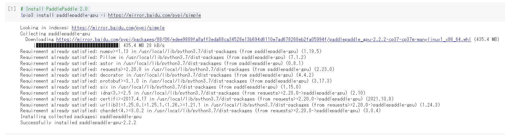
- PaddleOCR のインストール
https://github.com/PaddlePaddle/PaddleOCR/blob/release/2.4/doc/doc_en/quickstart_en.md に記載の手順による.
!pip3 install "paddleocr>=2.0.1"
- layout parser のインストール
!pip3 install -U https://paddleocr.bj.bcebos.com/whl/layoutparser-0.0.0-py3-none-any.whl
- PaddleOCR のソースコードやデータのダウンロード
あとで使用する.
%cd /content !rm -rf PaddleOCR !git clone https://github.com/PaddlePaddle/PaddleOCR %cd PaddleOCR
- 学習済みモデルのダウンロード
説明は https://github.com/PaddlePaddle/PaddleOCR/blob/release/2.4/doc/doc_en/models_list_en.md
- ch_PP-OCRv2_det_infer.tar, テキスト検知のモデル, Mobile & Server 用
- ch_ppocr_server_v2.0_det_infer.tar, テキスト検知のモデル, Mobile & Server 用
- en_number_mobile_v2.0_rec_slim_infer.tar, テキスト認識のモデル, Slim pruned and quantized lightweight model, supporting English and number recognition
- japan_mobile_v2.0_rec_infer.tar, テキスト認識のモデル, Lightweight model for Japanese recognition
- ch_ppocr_mobile_v2.0_cls_infer.tar, テキスト角分類のモデル
!curl -O https://paddleocr.bj.bcebos.com/PP-OCRv2/chinese/ch_PP-OCRv2_det_infer.tar !tar -xvf ch_PP-OCRv2_det_infer.tar !curl -O https://paddleocr.bj.bcebos.com/dygraph_v2.0/ch/ch_ppocr_server_v2.0_det_infer.tar !tar -xvf ch_ppocr_server_v2.0_det_infer.tar !curl -O https://paddleocr.bj.bcebos.com/dygraph_v2.0/multilingual/japan_mobile_v2.0_rec_infer.tar !tar -xvf japan_mobile_v2.0_rec_infer.tar !curl -O https://paddleocr.bj.bcebos.com/dygraph_v2.0/en/en_number_mobile_v2.0_rec_slim_infer.tar !tar -xvf en_number_mobile_v2.0_rec_slim_infer.tar !curl -O https://paddleocr.bj.bcebos.com/dygraph_v2.0/ch/ch_ppocr_mobile_v2.0_cls_infer.tar !tar -xvf ch_ppocr_mobile_v2.0_cls_infer.tar
- 横書きの日本語のテキスト検知 (text detection) の実行
https://github.com/PaddlePaddle/PaddleOCR/blob/release/2.4/doc/doc_en/inference_ppocr_en.md で説明の手順による.
!rm -f 1.jpg !wget https://www.kkaneko.jp/sample/textimage/1.jpg !python3 tools/infer/predict_det.py --image_dir="1.jpg" --det_model_dir="./ch_ppocr_server_v2.0_det_infer/" !cat ./inference_results/det_results.txt from PIL import Image Image.open('inference_results/det_res_1.jpg').show()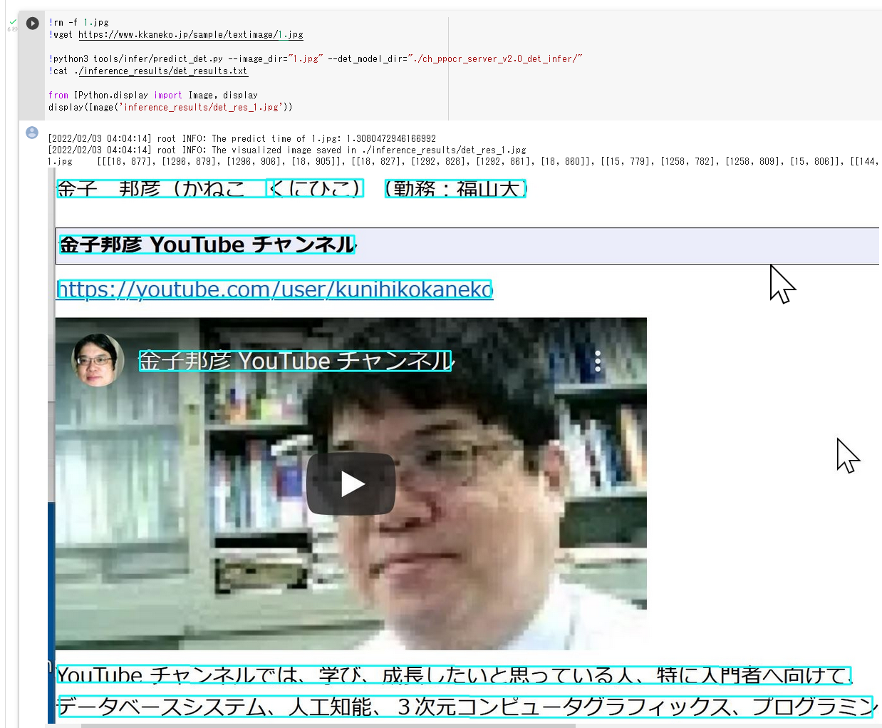
- 縦書きの日本語のテキスト検知 (text detection) の実行
https://github.com/PaddlePaddle/PaddleOCR/blob/release/2.4/doc/doc_en/inference_ppocr_en.md で説明の手順による.
!rm -f 2.jpg !wget https://www.kkaneko.jp/sample/textimage/2.jpg !python3 tools/infer/predict_det.py --image_dir="2.jpg" --det_model_dir="./ch_ppocr_server_v2.0_det_infer/" !cat ./inference_results/det_results.txt from PIL import Image Image.open('inference_results/det_res_2.jpg').show()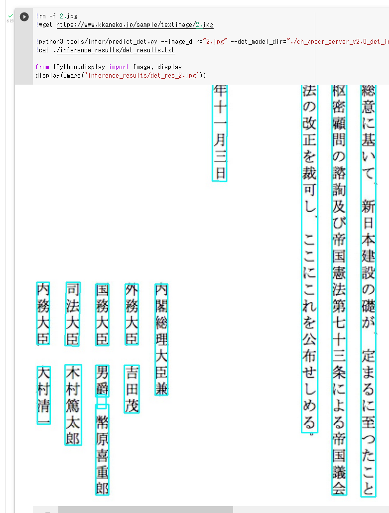
- 英語のテキスト検知 (text detection) の実行
https://github.com/PaddlePaddle/PaddleOCR/blob/release/2.4/doc/doc_en/inference_ppocr_en.md で説明の手順による.
!python3 tools/infer/predict_det.py --image_dir="./doc/imgs_en/img_12.jpg" --det_model_dir="./ch_ppocr_server_v2.0_det_infer/" !cat ./inference_results/det_results.txt from PIL import Image Image.open('inference_results/det_res_img_12.jpg').show()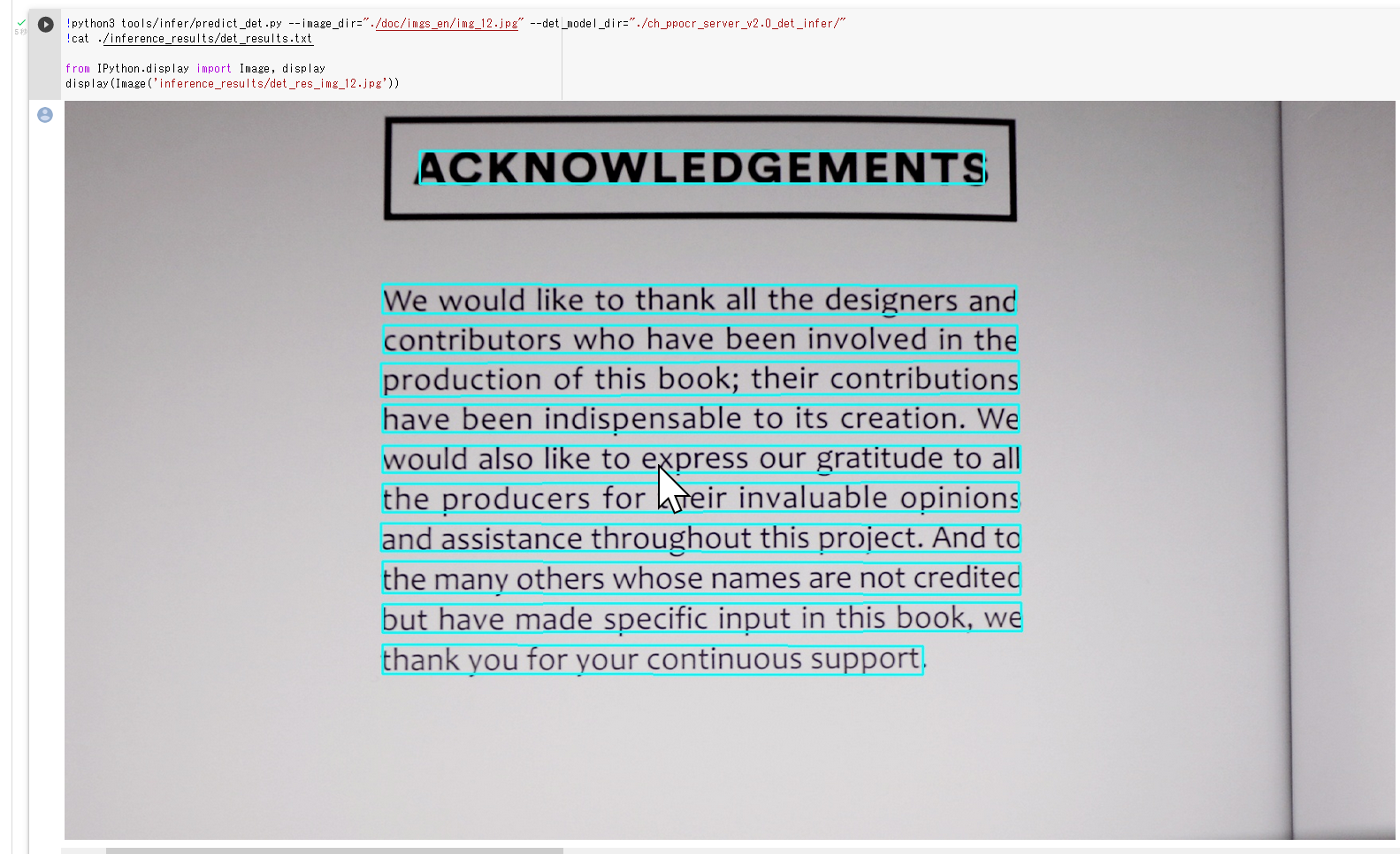
- 横書きの日本語のテキスト認識 (text recognition) の実行
https://github.com/PaddlePaddle/PaddleOCR/blob/release/2.4/doc/doc_en/inference_ppocr_en.md で説明の手順による.
!rm -f 1.jpg !wget https://www.kkaneko.jp/sample/textimage/1.jpg !python3 tools/infer/predict_system.py --image_dir="1.jpg" --det_model_dir="./ch_ppocr_server_v2.0_det_infer/" --cls_model_dir="./ch_ppocr_mobile_v2.0_cls_infer/" --rec_model_dir="japan_mobile_v2.0_rec_infer" --rec_char_dict_path="ppocr/utils/dict/japan_dict.txt" --vis_font_path="doc/fonts/japan.ttc" !cat ./inference_results/det_results.txt from PIL import Image Image.open('inference_results/1.jpg').show()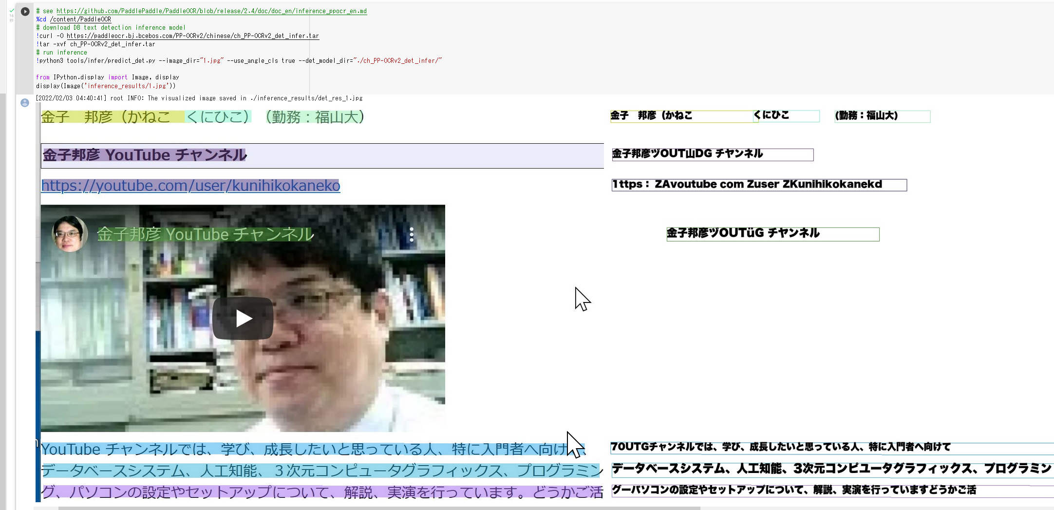
- 縦書きの日本語のテキスト認識 (text recognition) の実行
https://github.com/PaddlePaddle/PaddleOCR/blob/release/2.4/doc/doc_en/inference_ppocr_en.md で説明の手順による.
!rm -f 2.jpg !wget https://www.kkaneko.jp/sample/textimage/2.jpg !python3 tools/infer/predict_system.py --image_dir="2.jpg" --det_model_dir="./ch_ppocr_server_v2.0_det_infer/" --cls_model_dir="./ch_ppocr_mobile_v2.0_cls_infer/" --rec_model_dir="japan_mobile_v2.0_rec_infer" --rec_char_dict_path="ppocr/utils/dict/japan_dict.txt" --vis_font_path="doc/fonts/japan.ttc" !cat ./inference_results/det_results.txt from PIL import Image Image.open('inference_results/2.jpg').show()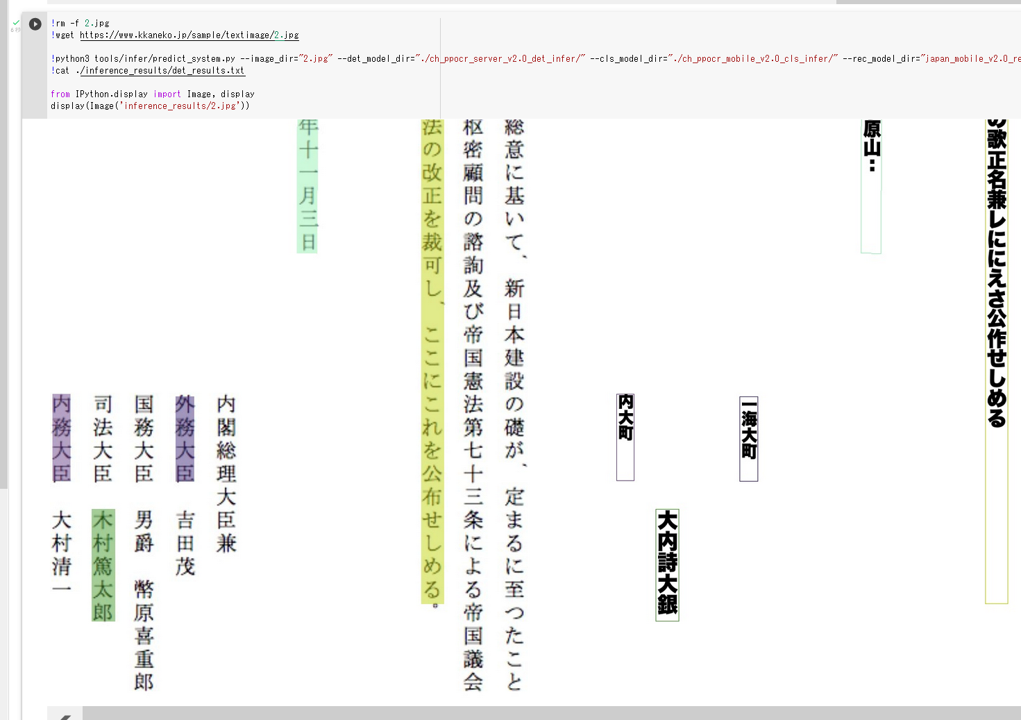
- 英語のテキスト認識 (text recognition) の実行
https://github.com/PaddlePaddle/PaddleOCR/blob/release/2.4/doc/doc_en/inference_ppocr_en.md で説明の手順による.
!python3 tools/infer/predict_system.py --image_dir="./doc/imgs_en/img_12.jpg" --det_model_dir="./ch_ppocr_server_v2.0_det_infer/" --cls_model_dir="./ch_ppocr_mobile_v2.0_cls_infer/" --rec_model_dir="en_number_mobile_v2.0_rec_slim_infer" --rec_char_dict_path="ppocr/utils/dict/en_dict.txt" from PIL import Image Image.open('inference_results/img_12.jpg').show()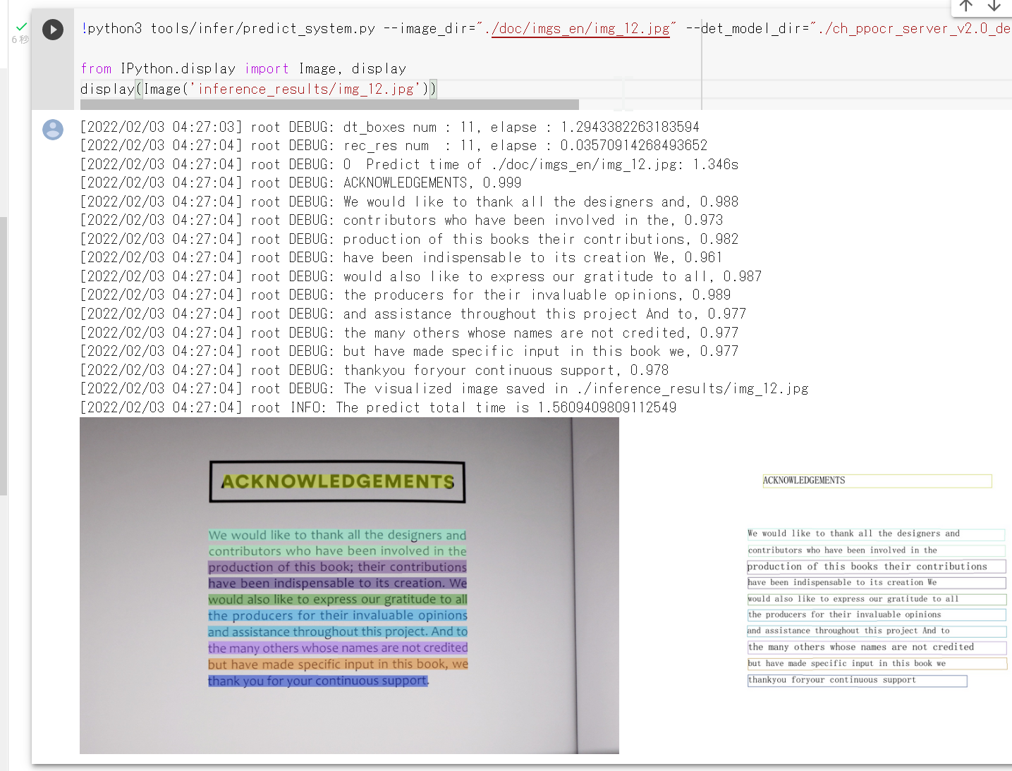
- 日本語のテキスト認識を行う Python プログラム
# see https://github.com/PaddlePaddle/PaddleOCR/blob/release/2.4/doc/doc_en/quickstart_en.md from paddleocr import PaddleOCR,draw_ocr # Paddleocr supports Chinese, English, French, German, Korean and Japanese. # You can set the parameter `lang` as `ch`, `en`, `fr`, `german`, `korean`, `japan` # to switch the language model in order. ocr = PaddleOCR(use_angle_cls=True, det_model_dir="./ch_ppocr_server_v2.0_det_infer/", cls_model_dir='./ch_ppocr_mobile_v2.0_cls_infer/', lang='japan') # need to run only once to download and load model into memory img_path = './2.jpg' result = ocr.ocr(img_path, cls=True) for line in result: print(line) # draw result from PIL import Image image = Image.open(img_path).convert('RGB') boxes = [line[0] for line in result] txts = [line[1][0] for line in result] scores = [line[1][1] for line in result] im_show = draw_ocr(image, boxes, txts, scores, font_path='./doc/fonts/japan.ttc') im_show = Image.fromarray(im_show) im_show.save('result.jpg') from PIL import Image Image.open('result.jpg').show()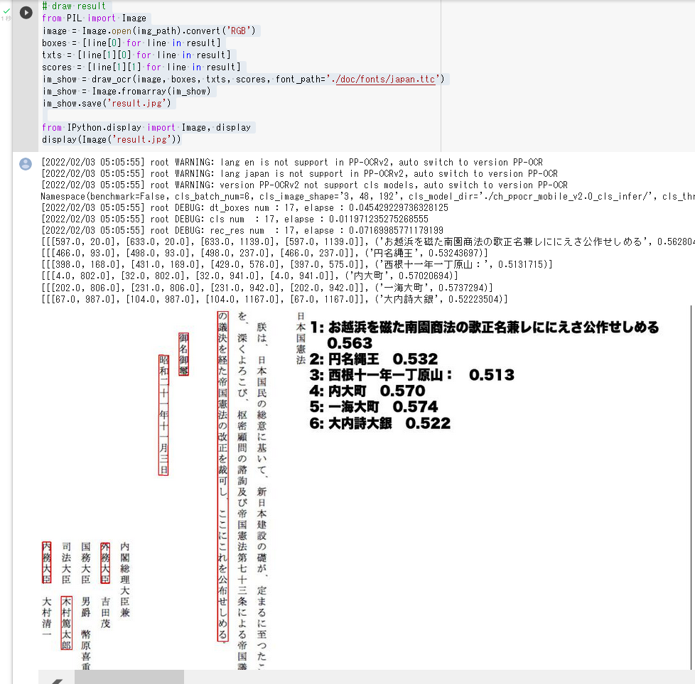
- テキスト検知 (text detection) の実行と,画像での結果の表示,英語の文書を使用
from paddleocr import PaddleOCR,draw_ocr # Paddleocr supports Chinese, English, French, German, Korean and Japanese. # You can set the parameter `lang` as `ch`, `en`, `fr`, `german`, `korean`, `japan` # to switch the language model in order. ocr = PaddleOCR(use_angle_cls=True, lang='en') # need to run only once to download and load model into memory img_path = './doc/imgs_en/img_12.jpg' result = ocr.ocr(img_path, cls=True) for line in result: print(line) # draw result from PIL import Image image = Image.open(img_path).convert('RGB') boxes = [line[0] for line in result] txts = [line[1][0] for line in result] scores = [line[1][1] for line in result] im_show = draw_ocr(image, boxes, txts, scores, font_path='./doc/fonts/simfang.ttf') im_show = Image.fromarray(im_show) im_show.save('result.jpg') from PIL import Image Image.open('result.jpg').show()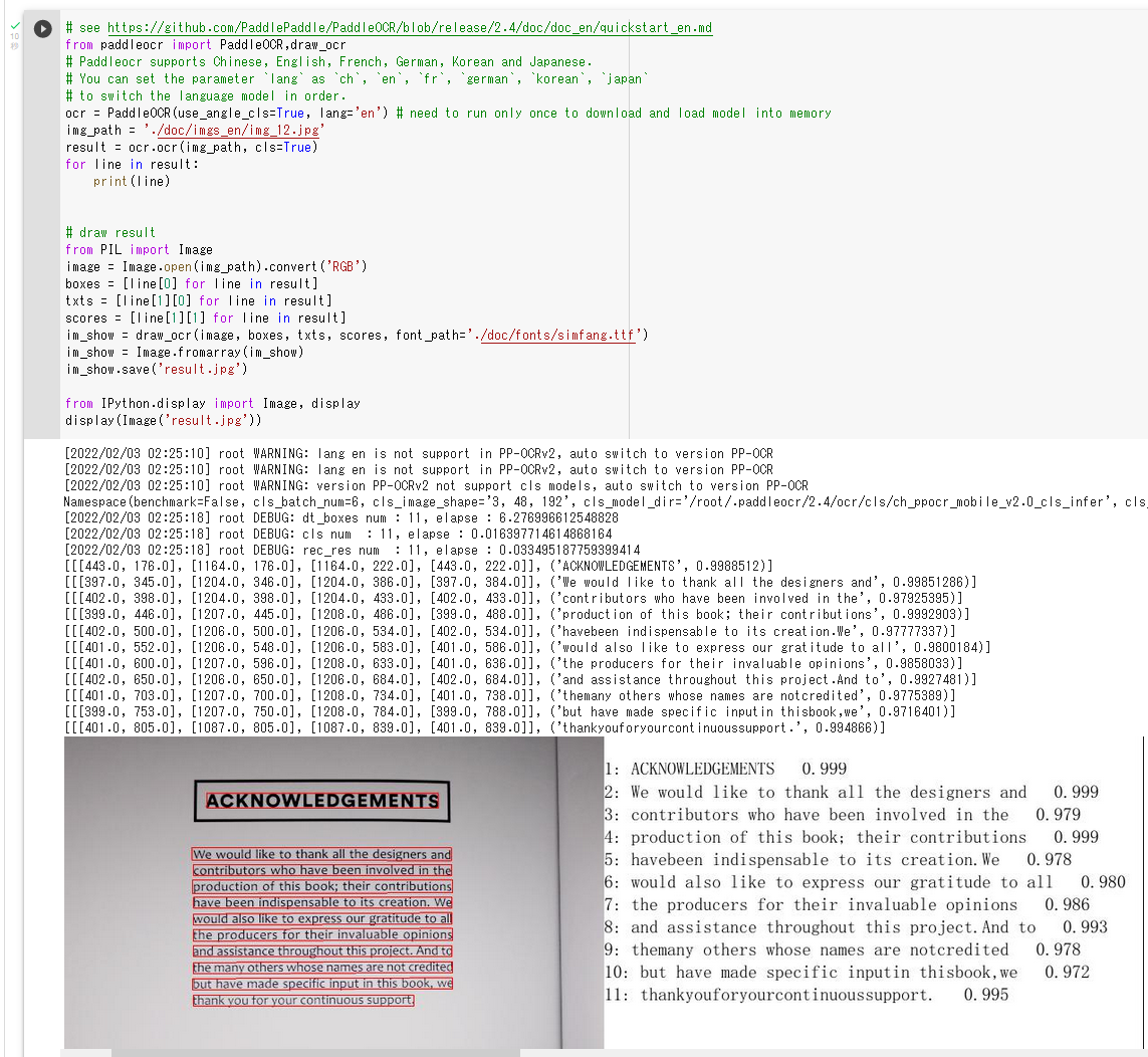
- 構造の読み取り
!paddleocr --image_dir ./doc/imgs_en/img_12.jpg --lang en --use_gpu false --type structure
OPT
OPT (Open Pre-Trained Transformer) は,事前学習済みの大規模言語モデル (large language model) である.GitHub のページでは,OPT-125M, OPT-350M, OPT-1.3B, OPT-2.7B, OPT-6.7B, OPT-13B, OPT-30B, OPT-66B, OPT-175B が公開されている.
【文献】
Susan Zhang, Stephen Roller, Naman Goyal, Mikel Artetxe, Moya Chen, Shuohui Chen, Christopher Dewan, Mona Diab, Xian Li, Xi Victoria Lin, Todor Mihaylov, Myle Ott, Sam Shleifer, Kurt Shuster, Daniel Simig, Punit Singh Koura, Anjali Sridhar, Tianlu Wang, Luke Zettlemoyer, OPT: Open Pre-trained Transformer Language Models, arXiv:2205.01068, 2022.
https://arxiv.org/pdf/2205.01068.pdf
【関連する外部ページ】
GitHub のページ: https://github.com/facebookresearch/metaseq/tree/main/projects/OPT
【関連項目】 FlexGen
Orbit
TensorFlow 2 で訓練ループのプログラムを書くときに利用できるソフトウェアである.
Orbit の GitHub のページ: https://github.com/tensorflow/models/tree/master/orbit
関連項目: TensorFlow
Oxford-IIIT ペット データセット
Oxford-IIIT ペット データセットは, 約200枚の画像と37の異なるカテゴリで構成されている. 主に犬と猫の画像とそれに対応するアノテーションデータが含まれており, 物体検出やセグメンテーションのタスクに利用できる.
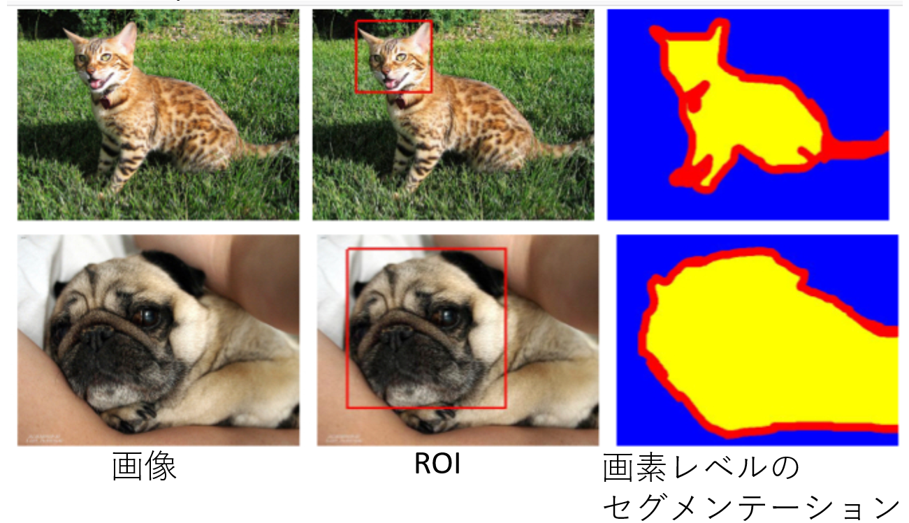
【関連する外部ページ】
Windows でのダウンロード手順
cd /d c:%HOMEPATH%
rmdir /s /q oxford3t
mkdir oxford3t
cd oxford3t
curl -L -O https://thor.robots.ox.ac.uk/~vgg/data/pets/images.tar.gz
curl -L -O https://thor.robots.ox.ac.uk/~vgg/data/pets/annotations.tar.gz
"c:\Program Files\7-Zip\7z.exe" x images.tar.gz
"c:\Program Files\7-Zip\7z.exe" x annotations.tar.gz
"c:\Program Files\7-Zip\7z.exe" x images.tar
"c:\Program Files\7-Zip\7z.exe" x annotations.tar
PANet (Path Aggregation Network)
物体検出とインスタンス・セグメンテーション (instance segmentation)のためのネットワークである. Mask R-CNN をもとに改善を行っている. PANet のネットワークは,FPN バックボーンののち, Bottom-up Path Augmentation を行い, Adaptive Feature Pooling を行っている.
COCO データセット, Cityscapes データセット, MVD データセットでの実験から,物体検出とインスタンス・セグメンテーション (instance segmentation)の精度が向上したとされている.
CSPNet の公式の実装 (GitHub) のページでは, PANetを用いた物体検出として, CSPDarknet53-PANet-SPP, CSPResNet50-PANet-SPP, CSPResNeXt50-PANet-SPP 等の実装が公開されている.
- 文献
Shu Liu, Lu Qi, Haifang Qin, Jianping Shi, Jiaya Jia, Path Aggregation Network for Instance Segmentation, CVPR 2018, also CoRR, https://arxiv.org/abs/1803.01534v4,
- PANet の公式の実装 (GitHub) のページ: https://github.com/ShuLiu1993/PANet
- YOLOv5 の GitHub のページ: https://github.com/ultralytics/yolov5
【関連項目】 Mask R-CNN, 物体検出, インスタンス・セグメンテーション (instance segmentation), YOLOv5
PARE
PARE は,3次元人体姿勢推定(3D human pose estimation)の技術である. オクルージョンの問題を解決するために, Part Attention REgressor (PARE) が提案されている. multi person tracker を用いて実装されており,画像の中に複数の人物がいても動くようになっている.
PARE のデモプログラムの実行結果を次に示す.
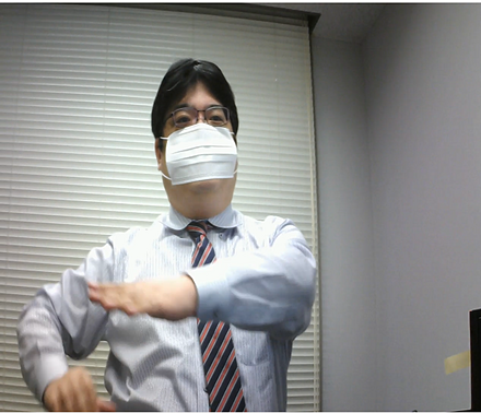
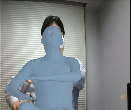
この実行結果を得るためのもととなる動画: kaneko_sample_video.mp4
実行結果の動画: kaneko_sample_video__result.mp4
- 文献
Kocabas, Muhammed and Huang, Chun-Hao P. and Hilliges, Otmar and Black, Michael J., PARE: Part Attention Regressor for {3D} Human Body Estimation, Proc. International Conference on Computer Vision (ICCV), also CoRR, abs/2104.08527v2, 2021.
- 公式のページ: https://pare.is.tue.mpg.de/
- 公式の GitHub のページ: https://github.com/mkocabas/PARE
- Papers with Code のページ: https://paperswithcode.com/paper/pare-part-attention-regressor-for-3d-human
【関連項目】 3D pose estimation, 3D human pose estimation, YOLOv3, multi person tracker
Google Colaboratory での PARE のインストールと事前学習済みモデルのダウンロードとデモの実行
次のコマンドやプログラムは Google Colaboratory で動く(コードセルを作り,実行する).
- Google Colaboratory で,ランタイムのタイプを GPU に設定する.
- 次を実行する.
!rm -rf PARE !git clone https://github.com/mkocabas/PARE.git %cd PARE !apt -y install libturbojpeg !pip3 uninstall -y torchtext panel datascience !pip3 install -U -r requirements.txt !source scripts/prepare_data.sh !python3 scripts/demo.py --vid_file data/sample_video.mp4 --output_folder logs/demo - 下図のように,/content/logs/demo/sample_video_ の下に結果ができる
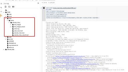
Ubuntu での PARE のインストールとデモの実行
前準備:事前に Python のインストール: 別項目で説明している.
- Ubuntu でインストールを行うには,次のコマンドを実行する.
# パッケージリストの情報を更新 sudo apt update sudo apt -y install git cd /usr/local sudo rm -rf PARE sudo git clone https://github.com/mkocabas/PARE.git sudo chown -R $USER PARE # システム Python の環境とは別の Python の仮想環境(システム Python を使用)を作成 sudo apt -y update sudo apt -y install python3-venv python3 -m venv ~/a source ~/a/bin/activate cd /usr/local/PARE sudo apt -y install libturbojpeg sed -i 's/opencv-python==4.1.1.26/opencv-python/g' requirements.txt pip install -U -r requirements.txt pip install -U numba - 事前学習済みモデルのダウンロード
source scripts/prepare_data.sh - デモの実行
python scripts/demo.py --vid_file data/sample_video.mp4 --output_folder logs/demo - 下のように,logs/demo/sample_video_ の下に結果ができる

出来た動画を表示すると,次のように表示される.
Pascal VOC (Pascal Visual Object Classes Challenge) データセット
Pascal VOC データセットは,アノテーション済みの画像データである. 機械学習での物体検出 ,画像分類,セマンティック・セグメンテーションに利用できるデータセットである. Pascal VOC 2007, Pascal VOC 2012 などいくつかの種類がある.
Pascal VOC 2012 データセット
- ピクセルレベルのセグメンテーションのアノテーション,バウンディングボックスのアノテーション,オブジェクトクラスのアノテーションが付いている.
- 学習用の1,464枚の画像,検証用の1,449枚の画像,その他のテストセットを含む
- オブジェクトのカテゴリ数: 20, その他,背景を表すカテゴリが 1.
vehicles, household, animals, and other: aeroplane, bicycle, boat, bus, car, motorbike, train, bottle, chair, dining table, potted plant, sofa, TV/monitor, bird, cat, cow, dog, horse, sheep, person
Pascal VOC データセットは次の URL で公開されているデータセット(オープンデータ)である.
http://host.robots.ox.ac.uk/pascal/VOC/
【関連情報】
- 文献
Everingham, M., Van Gool, L., Williams, C. K. I., Winn, J. and Zisserman, A., The Pascal Visual Object Classes (VOC) Challenge, International Journal of Computer Vision, 88(2), 303-338, 2010
- 文献
Everingham, M., Eslami, S. M. A., Van Gool, L., Williams, C. K. I., Winn, J. and Zisserman, A., The Pascal Visual Object Classes Challenge: A Retrospective, International Journal of Computer Vision, 111(1), 98-136, 2015.
- Pascal VOC の公式ページ: http://host.robots.ox.ac.uk/pascal/VOC/index.html
- Papers With Code の Pascal VOC データセットのページ: https://paperswithcode.com/dataset/pascal-voc
- PyTorch の Pascal VOC データセット: https://pytorch.org/vision/stable/datasets.html#torchvision.datasets.VOCSegmentation
【関連項目】 Detectron2, MMSegmentation, セマンティック・セグメンテーション (semantic segmentation), 画像分類, 物体検出
Photo Tourism データセット
Photo Tourism データセットは次の URL で公開されているデータセット(オープンデータ)である.
http://phototour.cs.washington.edu/datasets/
【関連情報】
- 文献
Noah Snavely, Steven M. Seitz, Richard Szeliski, "Photo tourism: Exploring photo collections in 3D," ACM Transactions on Graphics (SIGGRAPH Proceedings), 25(3), 2006, 835-846.
- 公式ページ: http://phototour.cs.washington.edu/patches/default.htm
- PyTorch の PhotoTour データセットの説明: https://pytorch.org/vision/stable/datasets.html#phototour
Places365 データセット
Places365 データセットは,シーンクラスに分類済みの画像データである. 機械学習での画像分類の学習や検証に利用できるデータセットである.
- 1000万枚の画像
- 434 のシーンクラス
- 2つのバージョン Places365-Standard と Places365-Challenge-2016 がある. Places365-Standardは,K=365個のシーンクラスからなる180万枚の学習画像と36000枚の検証画像. Places365-Challenge-2016は,新しい69個のシーンクラスを含む620万枚の学習画像が追加されている. (434個のシーンクラスからなる合計800万枚の学習画像).
Places365 データセットは次の URL で公開されているデータセット(オープンデータ)である.
【関連情報】
- B. Zhou, A. Lapedriza, A. Khosla, A. Oliva, and A. Torralba, Places: A 10 million Image Database for Scene Recognition, IEEE Transactions on Pattern Analysis and Machine Intelligence, 2017
- Papers With Code の Places365 データセットのページ: https://paperswithcode.com/dataset/places365
- PyTorch の Places365 データセット: https://pytorch.org/vision/stable/datasets.html#torchvision.datasets.Places365
- TensorFlow データセットの Places365 データセット: https://www.tensorflow.org/datasets/catalog/places365_small
PointCloudLibrary の3次元点群データ
https://github.com/PointCloudLibrary/data では, 3次元点群データ (3-D point cloud data) が公開されている(オープンデータである).
Windows では,次のような手順でダウンロードできる.
- Git のインストール: 別項目で説明している.
Git の公式ページ: https://git-scm.com/
- ダウンロード
mkdir /p c:\data cd c:\data mkdir PointCloudLibrary cd PointCloudLibrary git clone --recursive https://github.com/PointCloudLibrary/data echo git clone --recursive https://github.com/PointCloudLibrary/data > download.txt
Ubuntu では,次のようなコマンドでダウンロードできる.
cd /usr/local
sudo mkdir PointCloudLibrary
cd PointCloudLibrary
sudo git clone --recursive https://github.com/PointCloudLibrary/data
echo "git clone --recursive https://github.com/PointCloudLibrary/data" > download.sh
3次元点群データ (3-D point cloud data) を扱うには,MeshLab や CloudCompare が便利である.
PoseC3D
スケルトンベースの動作認識 (skeleton-based action recognition) の一手法である.2021年発表.
- 文献
Haodong Duan and Yue Zhao and Kai Chen and Dian Shao and Dahua Lin and Bo Dai, Revisiting Skeleton-based Action Recognition, arXiv, 2104.13586, 2021.
- MMAction2 の PoseC3D の説明ページ: https://github.com/open-mmlab/mmaction2/blob/master/configs/skeleton/posec3d/README.md
【関連項目】 MMAction2, スケルトンベースの動作認識 (skeleton-based action recognition), 動作認識 (action recognition)
pycocotools
pycocotools は,COCO データセットを Python から扱う機能を持ったソフトウェアである.
pycocotools の GitHub のページ: https://github.com/cocodataset/cocoapi/tree/master/PythonAPI/pycocotools
関連項目: COCO (Common Object in Context) データセット
pycocotools のリポジトリ
オリジナルの pycocotools から分岐 (fork) したリポジトリがある. Python 3 や Windows に対応.オリジナルの方は開発が休止しているようである.
pycocotools のインストール(Windows 上)
- Build Tools for Visual Studio 2022 のインストール: 別項目で説明している.
- Git のインストール: 別項目で説明している.
Git の公式ページ: https://git-scm.com/
- Python のインストール: 別項目で説明している.
- Windows では,コマンドプロンプトを管理者として実行
- pycocotools のインストール
python -m pip install -U cython python -m pip install "git+https://github.com/philferriere/cocoapi.git#egg=pycocotools&subdirectory=PythonAPI"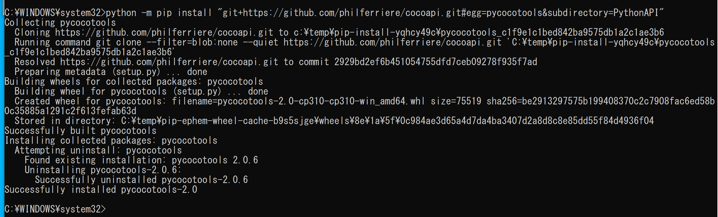
Ubuntu での pycocotools のインストール
Ubuntu でインストールを行うには,次のコマンドを実行する.
sudo pip3 install git+https://github.com/philferriere/cocoapi.git#subdirectory=PythonAPI
関連項目: COCO (Common Object in Context) データセット
PyCUDA
PyCUDA は NVIDIA CUDA API にアクセスできるようにするライブラリである.
pip を用いたインストールコマンド: python -m pip install -U pycuda
【関連する外部ページ】
【サイト内の関連ページ】
- PyCUDA のインストール,PyCUDA のプログラム例(Windows 上): 別ページ »で説明
【関連項目】 NVIDIA CUDA
PyMVPA
PyMVPAは,大規模データセットに対する統計的学習解析の 機能を持つ Pythonのパッケージである.
PyMVPA の URL: http://www.pymvpa.org/index.html
Pandas
TensorFlow などの機械学習フレームワークでは,入力として Pandas のデータ構造をサポートしていることが多い.
【関連項目】 Iris データセット
Pandas の表示
次のようなプログラムでは,displayを用いて,Pandas のデータフレームを整形して表示している.
from IPython.display import display
display(df)
Iris データセットを Pandas データフレームとしてロードし,画面表示するプログラム
次の Python プログラムは,Iris データセットのロードと確認表示を行う. Pandas データフレームの df にロードしている. 確認表示で display を用いている.
import pandas as pd
from sklearn.datasets import load_iris
from IPython.display import display
iris = load_iris()
df = pd.DataFrame(iris.data, columns=iris.feature_names)
df['species'] = iris.target_names[iris.target]
display(df)
Pandas での列の選択
次の Python プログラムでは,次のことを行っている.
- 複数の列の選択: df.iloc[:,0:4] は,0列目から4列分を得る.
- 1列の選択: df.iloc[:,4] は,4列目を得る.
import pandas as pd
from sklearn.datasets import load_iris
from IPython.display import display
iris = load_iris()
df = pd.DataFrame(iris.data, columns=iris.feature_names)
df['species'] = iris.target_names[iris.target]
display(df.iloc[:,0:4])
display(df.iloc[:,4])
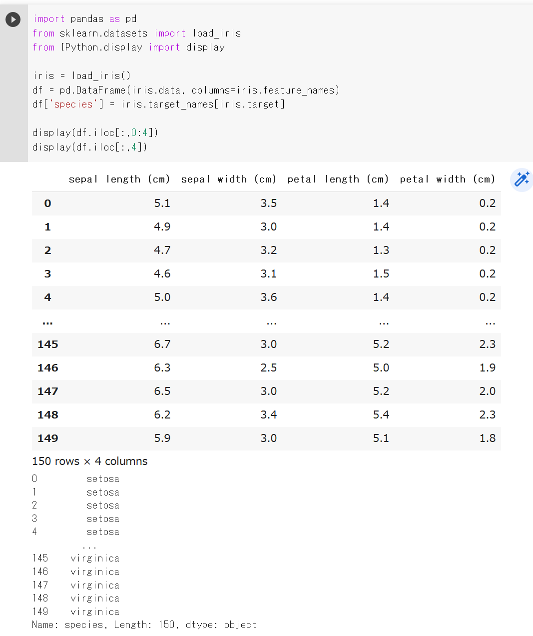
numpy.ndarray への変換
次の Python プログラムでは,to_numpy() を用いて, Pandas データフレームを numpy.ndarray へ変換している.
import pandas as pd
from sklearn.datasets import load_iris
from IPython.display import display
iris = load_iris()
df = pd.DataFrame(iris.data, columns=iris.feature_names)
df['species'] = iris.target_names[iris.target]
display(df.iloc[:,0:4].to_numpy())
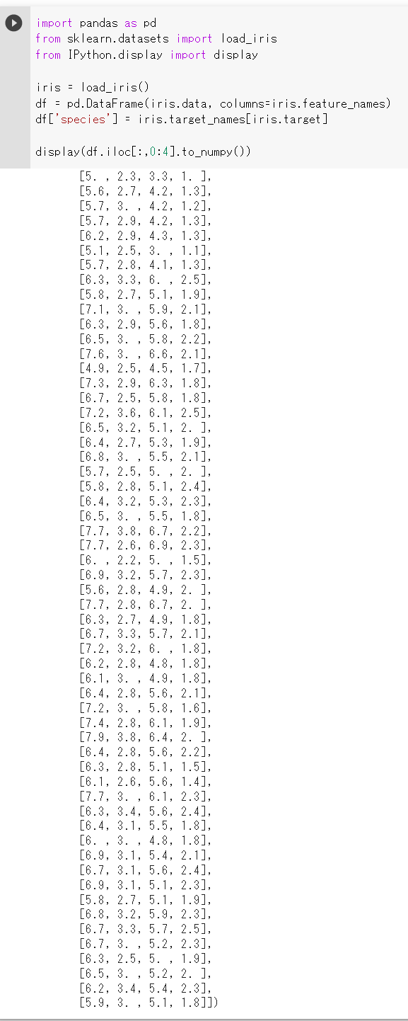
Pandas での繰り返し処理,選択
Pandas のある特定の列(カラム)のデータについて,処理を繰り返したいときの書き方.iris は Iris データセットである.
import pandas as pd
from sklearn.datasets import load_iris
from IPython.display import display
iris = load_iris()
df = pd.DataFrame(iris.data, columns=iris.feature_names)
df['species'] = iris.target_names[iris.target]
display([x * 10 for x in df['sepal length (cm)']])
Pandas のある特定の列(カラム)のデータについて,処理を繰り返すとき,ある条件(例えば 7 より大)のものだけ処理対象にしたいときの書き方
[x * 10 for x in iris['sepal_length'] if x > 7]
PyTorch
PyTorchは,ディープラーニングのフレームワークの 機能を持つ Pythonのパッケージである.
【関連する外部ページ】
- PyTorch の Web ページ: http://pytorch.org/
- GitHub: https://github.com/pytorch/pytorch
- GitHub: https://github.com/hughperkins/pytorch
- PyTorch のデータセット,モデル: https://github.com/pytorch/vision/
【関連項目】 Python のインストール,pip と setuptools の更新, Python 開発環境
PyTorch3D
公式ページ(GitHub): https://github.com/facebookresearch/pytorch3d
PyTorch-GAN のページ
Erik Linder-Norén により GitHub で公開されている PyTorch-GAN のページ.
URL は次のとおりである.
PyTorch-GAN のページ: https://github.com/eriklindernoren/PyTorch-GAN
PyTorch Geometric Temporal
【文献】
Benedek Rozemberczki and Paul Scherer and Yixuan He and George Panagopoulos and Alexander Riedel and Maria Astefanoaei and Oliver Kiss and Ferenc Beres and Guzman Lopez and Nicolas Collignon and Rik Sarkar, PyTorch Geometric Temporal: Spatiotemporal Signal Processing with Neural Machine Learning Models, Proceedings of the 30th ACM International Conference on Information and Knowledge Management, pp. 4564-4573, 2021.
【サイト内の関連ページ】
PyTorch Geometric Temporal のインストールと動作確認(予測)(Python,PyTorch を使用)(Windows 上)別ページ »で説明
【関連する外部ページ】
- GitHub のページ
https://github.com/benedekrozemberczki/pytorch_geometric_temporal
- 公式のドキュメント
https://pytorch-geometric-temporal.readthedocs.io/en/latest/
- 公式のサンプルプログラム
- 公式の Python ノートブックによるデモ
https://github.com/benedekrozemberczki/pytorch_geometric_temporal/tree/master/notebooks
【関連項目】 GNN (グラフニューラルネットワーク)
PyTorch, torchvision のモデル
URL: https://pytorch.org/vision/stable/models.html に説明がある.
【関連項目】 PyTorch, torchvision の DenseNet121 学習済みモデルのロード,画像分類のテスト実行, PyTorch, torchvision の DenseNet169 学習済みモデルのロード,画像分類のテスト実行, PyTorch, torchvision の MobileNetV3 large 学習済みモデルのロード,画像分類のテスト実行, PyTorch, torchvision の ResNet50 学習済みモデルのロード,画像分類のテスト実行, PyTorch, torchvision の ResNet101 学習済みモデルのロード,画像分類のテスト実行, PyTorch, torchvision の ResNet152 学習済みモデルのロード,画像分類のテスト実行, PyTorch, torchvision の ResNeXt50 32x4d 学習済みモデルのロード,画像分類のテスト実行, PyTorch, torchvision の ResNeXt101 32x8d 学習済みモデルのロード,画像分類のテスト実行, PyTorch, torchvision の Wide ResNet50 学習済みモデルのロード,画像分類のテスト実行, PyTorch, torchvision の Wide ResNet101 学習済みモデルのロード,画像分類のテスト実行, rwightman の PyTorch Image Models (TIMM)
Recognize Anything Model
画像タグ付けの学習は画像とテキストのペアを訓練データとして使用する. Recognize Anything Model(RAM)は,画像タグ付けのためのモデルで,手動でのアノテーションではなく,テキストのセマンティック解析を自動化することでラベルを取得することを特徴とする. Recognize Anything Model(RAM)のラベルシステムは,6,449の一般的なラベルを含んでいる. また,データエンジンは,欠落しているラベルを追加し,誤ったラベルをクリーニングするために使用される. データエンジンは既存のモデルを用いて追加のタグを生成し,画像内の特定のカテゴリに対応する領域を特定する.その後,同じカテゴリ内の領域を処理し,異常値を排除する. さらに,Recognize Anything Model(RAM)は画像タグ付けとキャプションのタスクを統合し,その結果,ゼロショット画像タグ付けを可能にしている.これにより,未見のカテゴリについての処理が可能になる.また,学習のコストを抑制するために,Recognize Anything Model(RAM)はオープンソースでアノテーションフリーのデータセットを使用する.これらの特性により,Recognize Anything Model(RAM)はゼロショットの画像タグ付けだけでなく,学習済みモデルを用いた画像タグ付けでも高い性能を示すとされる.これは,OpenImages V6,COCO,ADE20kなどの一連のベンチマークデータセットでの評価により裏付けられている.
【文献】 Recognize Anything: A Strong Image Tagging Model, 6 Jun 2023, Youcai Zhang, Xinyu Huang, Jinyu Ma, Zhaoyang Li, Zhaochuan Luo, Yanchun Xie, Yuzhuo Qin, Tong Luo, Yaqian Li, Shilong Liu, Yandong Guo, Lei Zhang.
https://arxiv.org/pdf/2306.03514v3.pdf
【サイト内の関連ページ】 Recognize Anything のインストールと動作確認(ゼロショットの画像タグ付け)(Python,PyTorch を使用)(Windows 上)
【関連する外部ページ】
- GitHub の公式ページ: https://github.com/xinyu1205/recognize-anything
- Papers with Code のページ: https://paperswithcode.com/paper/recognize-anything-a-strong-image-tagging
Real-ESRGAN
超解像 (super resolution) の一手法.2021 年発表.
【文献】
Xintao Wang and Liangbin Xie and Chao Dong and Ying Shan, Real-ESRGAN: Training Real-World Blind Super-Resolution with Pure Synthetic Data, International Conference on Computer Vision Workshops (ICCVW), https://arxiv.org/abs/2107.10833, 2021.
【関連する外部ページ】
- Real-ESRGAN の GitHub のページ: https://github.com/xinntao/Real-ESRGAN
- Real-ESRGAN のデモページ: https://colab.research.google.com/drive/1k2Zod6kSHEvraybHl50Lys0LerhyTMCo?usp=sharing#scrollTo=7IMD5vhOYp68
処理前の画像

処理結果
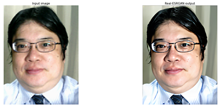
【関連項目】 APA, GAN (Generative Adversarial Network), image super resolution, video restoration, video super resolution, 超解像 (super resolution)
ReLU
ReLU (rectified linear unit) は,次の関数である.
f(x) = 0 for x < 0, f(x) = x for x >= 0
ReLUは,活性化関数としてよく使用されるもののうちの1つである. 活性化関数は,ニューロンの入力の合計から,そのニューロンの活性度の値を決めるためのものである. (他には,LReLU,シグモイド関数,ステップ関数,ソフトマックス関数などがある.)
Residual Networks (ResNets)
residual function (残余関数)を特徴とするニューラルネットワークである.
画像分類のための利用, 物体検出や セマンティック・セグメンテーションなどでのバックボーンでの利用などが行われている.
Residual Networks は DeepLabv3, Inception-v4, Inception-ResNet, ResNet50, ResNet101, ResNet152, その他の ResNet, ResNeXt, RetinaNet, SpineNet など,種々のモデルで使用されている.
- mask head アーキテクチャの論文
Vighnesh Birodkar, Zhichao Lu, Siyang Li, Vivek Rathod, Jonathan Huang, The surprising impact of mask-head architecture on novel class segmentation, 2021.
- SpineNet の論文
Xianzhi Du, Tsung-Yi Lin, Pengchong Jin, Golnaz Ghiasi, Mingxing Tan, Yin Cui, Quoc V. Le, Xiaodan Song, SpineNet: Learning Scale-Permuted Backbone for Recognition and Localization, CVPR 2020, 2020.
- semi-supervised learning に関する論文
Meta Pseudo Labels, Hieu Pham, Zihang Dai, Qizhe Xie, Minh-Thang Luong, Quoc V. Le, CVPR 2021, 2021.
- DeepLabv3 に関する論文
Liang-Chieh Chen, George Papandreou, Florian Schroff, Hartwig Adam, Rethinking Atrous Convolution for Semantic Image Segmentation, 2017.
- RetinaNet に関する論文
Tsung-Yi Lin, Priya Goyal, Ross Girshick, Kaiming He, Piotr Dollár, Focal Loss for Dense Object Detection, ICCV 2017, 2017.
- Inception-v4, Inception-ResNet に関する論文
Christian Szegedy, Sergey Ioffe, Vincent Vanhoucke, Alex Alemi, Inception-v4, Inception-ResNet and the Impact of Residual Connections on Learning, 2016.
- ResNet18, ResNet34, ResNet50, ResNet101, ResNet152 に関する論文
Kaiming He, Xiangyu Zhang, Shaoqing Ren, Jian Sun, Deep Residual Learning for Image Recognition, CVPR 2016, 2016.
- Papers with Code のページ: https://paperswithcode.com/method/resnet
【関連項目】 DeepLabv3, ResNet50, ResNet101, ResNet152, その他の ResNet, ResNeXt, RetinaNet, セマンティック・セグメンテーション (semantic segmentation), 画像分類, 物体検出
ResNet50, ResNet101, ResNet152, その他の ResNet
Keras の ResNet50 を用いて ResNet50 のモデルを作成するプログラムは次のようになる. 「weights=None」を指定することにより,最初,重みをランダムに設定する.
m = tf.keras.applications.resnet50.ResNet50(input_shape=INPUT_SHAPE, weights=None, classes=NUM_CLASSES)
CoRR, abs/1512.03385
Keras の応用のページ: https://keras.io/api/applications/
【関連項目】 Residual Networks (ResNets), モデル, 画像分類
PyTorch, torchvision の ResNet50 学習済みモデルのロード,画像分類のテスト実行
Google Colab あるいはパソコン(Windows あるいは Linux)を使用.
- 前準備
前準備として,Python のインストール: 別項目で説明している. PyTorch のインストール を行う.
Google Colaboratory では, Python, PyTorch はインストール済みなので,インストール操作は不要.次に,pip を用いて,pillow のインストールを行う.
pip install -U pillow - ImageNet データセット で学習済みのResNet50 モデルのロード
PyTorch, torchvision のモデルについては: https://pytorch.org/vision/stable/models.html に説明がある.
import torch import torchvision.models as models device = torch.device('cuda' if torch.cuda.is_available() else 'cpu') m = models.resnet50(pretrained=True).to(device) - 画像分類したい画像ファイルのダウンロードとロードと確認表示
from PIL import Image import requests from IPython.display import display # ダウンロードとロード url = 'https://github.com/pytorch/hub/raw/master/images/dog.jpg' response = requests.get(url) img = Image.open(requests.get(url, stream=True).raw) # 確認表示 display(img)
- 画像の前処理.PyTorch で扱えるようにするため.
from PIL import Image from torchvision import transforms img = Image.open(filename) preprocess = transforms.Compose([ transforms.Resize(256), transforms.CenterCrop(224), transforms.ToTensor(), transforms.Normalize(mean=[0.485, 0.456, 0.406], std=[0.229, 0.224, 0.225]), ]) input_tensor = preprocess(img) input_batch = input_tensor.unsqueeze(0) - 推論 (inference) の実行
「m.eval()」は,推論を行うときのためのものである.これを行わないと訓練(学習)が行われる.
import torch if torch.cuda.is_available(): input_batch = input_batch.to('cuda') m.eval() with torch.no_grad(): output = m(input_batch) - 結果の表示
import urllib url, filename = ("https://raw.githubusercontent.com/pytorch/hub/master/imagenet_classes.txt", "imagenet_classes.txt") try: urllib.URLopener().retrieve(url, filename) except: urllib.request.urlretrieve(url, filename) with open("imagenet_classes.txt", "r") as f: categories = [s.strip() for s in f.readlines()] # The output has unnormalized scores. To get probabilities, you can run a softmax on it. probabilities = torch.nn.functional.softmax(output[0], dim=0) print(probabilities) top5_prob, top5_catid = torch.topk(probabilities, 5) for i in range(top5_prob.size(0)): print(categories[top5_catid[i]], top5_prob[i].item())Google Colaboratory での結果
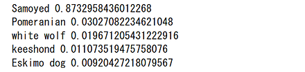
Windows での結果
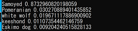
Linux での結果
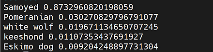
PyTorch, torchvision の ResNet101 学習済みモデルのロード,画像分類のテスト実行
Google Colab あるいはパソコン(Windows あるいは Linux)を使用.
- 前準備
前準備として,Python のインストール: 別項目で説明している. PyTorch のインストール を行う.
Google Colaboratory では, Python, PyTorch はインストール済みなので,インストール操作は不要.次に,pip を用いて,pillow のインストールを行う.
pip install -U pillow - ImageNet データセット で学習済みのResNet101 モデルのロード
PyTorch, torchvision のモデルについては: https://pytorch.org/vision/stable/models.html に説明がある.
import torch import torchvision.models as models device = torch.device('cuda' if torch.cuda.is_available() else 'cpu') m = models.resnet101(pretrained=True).to(device) - 画像分類したい画像ファイルのダウンロードとロードと確認表示
from PIL import Image import requests from IPython.display import display # ダウンロードとロード url = 'https://github.com/pytorch/hub/raw/master/images/dog.jpg' response = requests.get(url) img = Image.open(requests.get(url, stream=True).raw) # 確認表示 display(img)
- 画像の前処理.PyTorch で扱えるようにするため.
from PIL import Image from torchvision import transforms img = Image.open(filename) preprocess = transforms.Compose([ transforms.Resize(256), transforms.CenterCrop(224), transforms.ToTensor(), transforms.Normalize(mean=[0.485, 0.456, 0.406], std=[0.229, 0.224, 0.225]), ]) input_tensor = preprocess(img) input_batch = input_tensor.unsqueeze(0) - 推論 (inference) の実行
「m.eval()」は,推論を行うときのためのものである.これを行わないと訓練(学習)が行われる.
import torch if torch.cuda.is_available(): input_batch = input_batch.to('cuda') m.eval() with torch.no_grad(): output = m(input_batch) - 結果の表示
import urllib url, filename = ("https://raw.githubusercontent.com/pytorch/hub/master/imagenet_classes.txt", "imagenet_classes.txt") try: urllib.URLopener().retrieve(url, filename) except: urllib.request.urlretrieve(url, filename) with open("imagenet_classes.txt", "r") as f: categories = [s.strip() for s in f.readlines()] # The output has unnormalized scores. To get probabilities, you can run a softmax on it. probabilities = torch.nn.functional.softmax(output[0], dim=0) print(probabilities) top5_prob, top5_catid = torch.topk(probabilities, 5) for i in range(top5_prob.size(0)): print(categories[top5_catid[i]], top5_prob[i].item())Google Colaboratory での結果
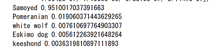
Windows での結果
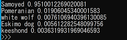
Linux での結果
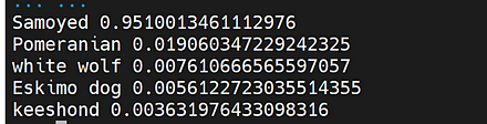
PyTorch, torchvision の ResNet152 学習済みモデルのロード,画像分類のテスト実行
Google Colab あるいはパソコン(Windows あるいは Linux)を使用.
- 前準備
前準備として,Python のインストール: 別項目で説明している. PyTorch のインストール を行う.
Google Colaboratory では, Python, PyTorch はインストール済みなので,インストール操作は不要.次に,pip を用いて,pillow のインストールを行う.
pip install -U pillow - ImageNet データセット で学習済みのResNet152 モデルのロード
PyTorch, torchvision のモデルについては: https://pytorch.org/vision/stable/models.html に説明がある.
import torch import torchvision.models as models device = torch.device('cuda' if torch.cuda.is_available() else 'cpu') m = models.resnet152(pretrained=True).to(device) - 画像分類したい画像ファイルのダウンロードとロードと確認表示
from PIL import Image import requests from IPython.display import display # ダウンロードとロード url = 'https://github.com/pytorch/hub/raw/master/images/dog.jpg' response = requests.get(url) img = Image.open(requests.get(url, stream=True).raw) # 確認表示 display(img)
- 画像の前処理.PyTorch で扱えるようにするため.
from PIL import Image from torchvision import transforms img = Image.open(filename) preprocess = transforms.Compose([ transforms.Resize(256), transforms.CenterCrop(224), transforms.ToTensor(), transforms.Normalize(mean=[0.485, 0.456, 0.406], std=[0.229, 0.224, 0.225]), ]) input_tensor = preprocess(img) input_batch = input_tensor.unsqueeze(0) - 推論 (inference) の実行
「m.eval()」は,推論を行うときのためのものである.これを行わないと訓練(学習)が行われる.
import torch if torch.cuda.is_available(): input_batch = input_batch.to('cuda') m.eval() with torch.no_grad(): output = m(input_batch) - 結果の表示
import urllib url, filename = ("https://raw.githubusercontent.com/pytorch/hub/master/imagenet_classes.txt", "imagenet_classes.txt") try: urllib.URLopener().retrieve(url, filename) except: urllib.request.urlretrieve(url, filename) with open("imagenet_classes.txt", "r") as f: categories = [s.strip() for s in f.readlines()] # The output has unnormalized scores. To get probabilities, you can run a softmax on it. probabilities = torch.nn.functional.softmax(output[0], dim=0) print(probabilities) top5_prob, top5_catid = torch.topk(probabilities, 5) for i in range(top5_prob.size(0)): print(categories[top5_catid[i]], top5_prob[i].item())Google Colaboratory での結果
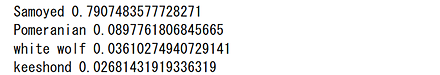
Windows での結果
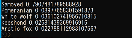
Linux での結果
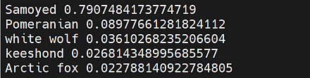
ResNeXt
ResNeXt は,ResNet の residual unit で grouped conv3x3 を使うとともに,conv1x1 の次元削減率を抑制することにより,速度を低下させず,精度を向上させるものである.
物体検出や セマンティック・セグメンテーションなどでのバックボーンでの利用も行われている.
- 文献
Saining Xie, Ross B. Girshick, Piotr Doll{\'{a}}r, Zhuowen Tu, Kaiming He, Aggregated Residual Transformations for Deep Neural Networks, CoRR, abs/1611.05431, 2016.
- Papers with Code のページ: https://paperswithcode.com/model/resnext
- PyTorch HUB のページ: https://pytorch.org/hub/pytorch_vision_resnext/
【関連項目】 PyTorch, torchvision のモデル, Residual Networks (ResNets), SE ResNeXt, モデル, 画像分類
PyTorch, torchvision の ResNeXt50 32x4d 学習済みモデルのロード,画像分類のテスト実行
Google Colab あるいはパソコン(Windows あるいは Linux)を使用.
- 前準備
前準備として,Python のインストール: 別項目で説明している. PyTorch のインストール を行う.
Google Colaboratory では, Python, PyTorch はインストール済みなので,インストール操作は不要.次に,pip を用いて,pillow のインストールを行う.
pip install -U pillow - ImageNet データセット で学習済みのResNeXt50 32x4d モデルのロード
PyTorch, torchvision のモデルについては: https://pytorch.org/vision/stable/models.html に説明がある.
import torch import torchvision.models as models device = torch.device('cuda' if torch.cuda.is_available() else 'cpu') m = models.resnext50_32x4d(pretrained=True).to(device) - 画像分類したい画像ファイルのダウンロードとロードと確認表示
from PIL import Image import requests from IPython.display import display # ダウンロードとロード url = 'https://github.com/pytorch/hub/raw/master/images/dog.jpg' response = requests.get(url) img = Image.open(requests.get(url, stream=True).raw) # 確認表示 display(img)
- 画像の前処理.PyTorch で扱えるようにするため.
from PIL import Image from torchvision import transforms img = Image.open(filename) preprocess = transforms.Compose([ transforms.Resize(256), transforms.CenterCrop(224), transforms.ToTensor(), transforms.Normalize(mean=[0.485, 0.456, 0.406], std=[0.229, 0.224, 0.225]), ]) input_tensor = preprocess(img) input_batch = input_tensor.unsqueeze(0) - 推論 (inference) の実行
「m.eval()」は,推論を行うときのためのものである.これを行わないと訓練(学習)が行われる.
import torch if torch.cuda.is_available(): input_batch = input_batch.to('cuda') m.eval() with torch.no_grad(): output = m(input_batch) - 結果の表示
import urllib url, filename = ("https://raw.githubusercontent.com/pytorch/hub/master/imagenet_classes.txt", "imagenet_classes.txt") try: urllib.URLopener().retrieve(url, filename) except: urllib.request.urlretrieve(url, filename) with open("imagenet_classes.txt", "r") as f: categories = [s.strip() for s in f.readlines()] # The output has unnormalized scores. To get probabilities, you can run a softmax on it. probabilities = torch.nn.functional.softmax(output[0], dim=0) print(probabilities) top5_prob, top5_catid = torch.topk(probabilities, 5) for i in range(top5_prob.size(0)): print(categories[top5_catid[i]], top5_prob[i].item())Google Colaboratory での結果
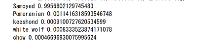
Windows での結果
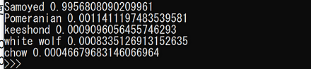
Linux での結果
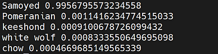
PyTorch, torchvision の ResNeXt101 32x8d 学習済みモデルのロード,画像分類のテスト実行
Google Colab あるいはパソコン(Windows あるいは Linux)を使用.
- 前準備
前準備として,Python のインストール: 別項目で説明している. PyTorch のインストール を行う.
Google Colaboratory では, Python, PyTorch はインストール済みなので,インストール操作は不要.次に,pip を用いて,pillow のインストールを行う.
pip install -U pillow - ImageNet データセット で学習済みのResNeXt101 32x8d モデルのロード
PyTorch, torchvision のモデルについては: https://pytorch.org/vision/stable/models.html に説明がある.
import torch import torchvision.models as models device = torch.device('cuda' if torch.cuda.is_available() else 'cpu') m = models.resnext101_32x8d(pretrained=True).to(device) - 画像分類したい画像ファイルのダウンロードとロードと確認表示
from PIL import Image import requests from IPython.display import display # ダウンロードとロード url = 'https://github.com/pytorch/hub/raw/master/images/dog.jpg' response = requests.get(url) img = Image.open(requests.get(url, stream=True).raw) # 確認表示 display(img)
- 画像の前処理.PyTorch で扱えるようにするため.
from PIL import Image from torchvision import transforms img = Image.open(filename) preprocess = transforms.Compose([ transforms.Resize(256), transforms.CenterCrop(224), transforms.ToTensor(), transforms.Normalize(mean=[0.485, 0.456, 0.406], std=[0.229, 0.224, 0.225]), ]) input_tensor = preprocess(img) input_batch = input_tensor.unsqueeze(0) - 推論 (inference) の実行
「m.eval()」は,推論を行うときのためのものである.これを行わないと訓練(学習)が行われる.
import torch if torch.cuda.is_available(): input_batch = input_batch.to('cuda') m.eval() with torch.no_grad(): output = m(input_batch) - 結果の表示
import urllib url, filename = ("https://raw.githubusercontent.com/pytorch/hub/master/imagenet_classes.txt", "imagenet_classes.txt") try: urllib.URLopener().retrieve(url, filename) except: urllib.request.urlretrieve(url, filename) with open("imagenet_classes.txt", "r") as f: categories = [s.strip() for s in f.readlines()] # The output has unnormalized scores. To get probabilities, you can run a softmax on it. probabilities = torch.nn.functional.softmax(output[0], dim=0) print(probabilities) top5_prob, top5_catid = torch.topk(probabilities, 5) for i in range(top5_prob.size(0)): print(categories[top5_catid[i]], top5_prob[i].item())Google Colaboratory での結果
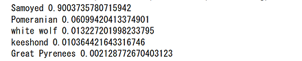
Windows での結果
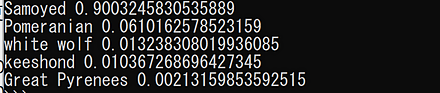
Linux での結果
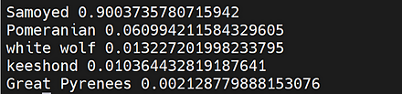
RetinaNet
focal loss 関数を特徴とする物体検出のモデルである.
- 文献
Lin, Tsung-Yi and Goyal, Priya and Girshick, Ross and He, Kaiming and Doll\'ar, Piotr, Focal loss for dense object detection, Proceedings of the IEEE international conference on computer vision, also CoRR, abs/1708.02002v2, 2017.
- 公式のソースコード (GitHub): https://github.com/facebookresearch/detectron
- Papers with Code のページ: https://paperswithcode.com/method/retinanet
- TensorFlow のモデル: https://github.com/tensorflow/models
- Detectron2: https://github.com/facebookresearch/detectron2, Detectron2 のチュートリアル: https://colab.research.google.com/drive/16jcaJoc6bCFAQ96jDe2HwtXj7BMD_-m5
- OpenMMLab の mmdetection: https://github.com/open-mmlab/mmdetection
【関連項目】 AlexeyAB darknet, Detectron, Detectron2, OpenMMLab, MMDetection, Residual Networks (ResNets), SpineNet, TensorFlow, YOLOv3, モデル, 物体検出
Reuters newswire topics データセット
Reuters newswire topics データセットは,公開されているデータセット(オープンデータ)である.
Reuters newswire topics データセットは,次のプログラムでロードできる.
from tensorflow.keras.datasets import reuters
(x_train, y_train), (x_test, y_test) = reuters.load_data()
【関連項目】 Keras に付属のデータセット
RNN (recurrent neural network)
ある層でのニューロンでの結果を,1つ前の層が受け取ったり, その層が受け取ったりするようにニューラルネットワークを作る場合もある. そのようなニューラルネットワークを「リカレントニューラルネットワーク」という. リカレントニューラルネットワークは,フィードフォワードではない. リカレントニューラルネットワークでは,前回の実行時での結果の一部が,次の実行に反映される.
【関連項目】 GRU (Gated Recurrent Neural Networks), LSTM (Long Short-Term Memory), フィードフォワード
rwightman の PyTorch Image Models (TIMM)
rwightman の PyTorch Image Models (TIMM) は, 画像分類の機能を持つライブラリである. 300以上の事前学習済みの画像分類モデルを簡単に利用することができる. ImageNet などのデータセットを用いた学習を簡単に行えるためのスクリプトも提供される. 事前学習済みの画像分類モデルを,自分自身のデータを用いてファインチューニング (fine tuning) を行うことを簡単に行える スクリプトも提供される.
学習,検証,推論を行うスクリプトは, https://github.com/rwightman/pytorch-image-models で説明が行われている.
- 公式の GitHub のページ: https://github.com/rwightman/pytorch-image-models
- rwightman の PyTorch Image Models (TIMM) の画像分類モデルの説明(Papers With Code 内): https://paperswithcode.com/lib/timm
- Papers with Code の URL: https://paperswithcode.com/lib/timm
【関連項目】 PyTorch, torchvision のモデル, モデル, 画像分類 (image classification)
R システム
R システムは,統計計算とグラフィックスのソフトウェアで,多数の機能を持つ. R システムの詳細は,そのホームページ https://www.r-project.org/ に記載されている.
【関連する外部ページ】 R システムの CRAN の URL: https://cran.r-project.org/
【サイト内の主な R 関連ページ】
- R システムの機能
- Windows での R システムのインストール: 別ページ »で説明
- Ubuntu での R システムのインストール: 別ページ »で説明
- R システムのプログラム例: 別ページ »にまとめ
- データシステム演習(R システム,Shiny を使用): 別ページ »にまとめ
- データサイエンス演習(R システムを使用): 別ページで説明している.
R システムの運用(パッケージのインストール,タスク・ビューのインストール,パッケージの更新など)
- CRAN ミラーサイトの選択
chooseCRANmirror() - パッケージのインストール(メニューから指定)
utils:::menuInstallPkgs() - パッケージのインストール(パッケージ名を指定)
install.packages("<パッケージ名>") - タスク・ビュー Cluster のインストール
タスク・ビューの詳細については,CRAN Task View のページ: https://cran.r-project.org/web/views/
options(repos="http://cran.rstudio.com") install.packages("ctv", repos="http://cran.rstudio.com/") library(ctv) install.views("Cluster")bioclite のインストール
source("http://bioconductor.org/biocLite.R") biocLite(groupName="all") - すべてのパッケージの更新
update.packages(checkBuilt=TRUE, ask=FALSE)
【関連項目】 R データセット
R データセット (Rdatasets)
R データセット (Rdatasets)は, 1700 を超えるデータセットの集まりである.
R データセット (Rdatasets) の URL: https://vincentarelbundock.github.io/Rdatasets
Python で R データセット (Rdatasets)を用いる場合には, 次のように,データ名とパッケージを指定する. データ名とパッケージは,https://vincentarelbundock.github.io/Rdatasets で確認できる.
import statsmodels.api as sm
df = sm.datasets.get_rdataset("Duncan", "carData")
print(df.__doc__)
print(df.data)
Segment Anything Model (SAM)
Segment Anything(SA)は,画像セグメンテーションのための基盤モデルを構築することを目的としたプロジェクトである.このプロジェクトでは,新しいデータ分布とタスクに一般化できるプロンプト可能なセグメンテーションモデルSegment Anything Model(SAM)が開発された.Segment Anything Model(SAM)はゼロショットでのセグメンテーションが可能である.さらに,1100万枚以上の画像と,それらの画像に対する10億以上のマスクを含むセグメンテーションデータセットSA-1Bデータセットが構築された.
【文献】
Alexander Kirillov, Eric Mintun, Nikhila Ravi, Hanzi Mao, Chloe Rolland, Laura Gustafson, Tete Xiao, Spencer Whitehead, Alex Berg, Wan-Yen Lo, Piotr Dollar, Ross Girshick, Segment Anything, arXiv:2304.02643, 2023.
https://arxiv.org/pdf/2304.02643v1.pdf
【サイト内の関連ページ】
- ゼロショットのセグメンテーション(Segment Anything Model,Python,PyTorch を使用)(Windows 上): 別ページ »で説明
【関連する外部ページ】
- 公式の GitHub ページ: https://github.com/facebookresearch/segment-anything
- Segment Anything のオンラインデモ: https://segment-anything.com/demo#
- Papers with Code のページ: https://paperswithcode.com/paper/segment-anything
【関連項目】 HQ-SAM (Segment Anything in High Quality)
SBU データセット
SBU データセットは,影画像に関するデータセットである. 機械学習での影検出の学習や検証に利用できるデータセットである.
SBU データセットは,次の URL で公開されているデータセット(オープンデータ)である.
SBU データセット の URL: https://www3.cs.stonybrook.edu/~cvl/projects/shadow_noisy_label/index.html
【関連情報】
- 文献
Large-scale Training of Shadow Detectors with Noisily-Annotated Shadow Examples, Vicente, T.F.Y., Hou, L., Yu, C.-P., Hoai, M., Samaras, D., Proceedings of European Conference on Computer Vision (ECCV), 2016.
- PyTorch の SBU データセット: https://pytorch.org/vision/stable/datasets.html
scikit-learn
scikit-learnは,分類,回帰,クラスタリング,次元削減,Model selection などの機械学習の 機能を持つ Pythonのパッケージである.
scikit-learn の URL: https://scikit-learn.org/stable/
SCRFD (Sample and Computation Redistribution for Face Detection)
SCRFD は顔検出の手法である. TinaFace に対しては,画像が低解像度のとき速く処理できない,そして,一般の物体認識法である RetinaNet をベースに設計されているために,顔検出 (face detection)に用いるには冗長であったり,最適化しつくし切れていない という見解が示されているようである. WIDER FACE データセット の HARD レベルの顔は,78.83% の顔が 32x32 画素よりも小さいということも示されている. SCRFD では,探索空間の削減のために, sample redistribution と computation redistribution を 2段階で行う方法が提案されている. WIDER FACE データセット による実験結果では,TinaFace を精度と性能で上回るとされている.
- 文献
Jia Guo, Jiankang Deng, Alexandros Lattas, Stefanos Zafeiriou, Sample and Computation Redistribution for Efficient Face Detection, 2021. arXiv:2105.04714 [cs.CV]
- Papers with Code のページ: https://paperswithcode.com/paper/sample-and-computation-redistribution-for
- ソースコード: https://github.com/deepinsight/insightface
- SCRFD の事前学習済みモデル(InsightFace 内): https://github.com/deepinsight/insightface/tree/master/detection/scrfd
- SCRFD の実行については,InsightFace の項目で説明している.
【関連項目】 InsightFace, RetinaNet, TinaFace, 顔検出 (face detection)
Stable Diffusion XL (SDXL)
Stable Diffusion XL (SDXL)は,Stability AI によって開発された Diffusion ベースの text-to-image の画像生成モデルである. SDXL は Stable Diffusion with Larger UNet Backbone の略称である.
SDXL は,以前の Stable Diffusion モデルと比較して,UNet バックボーンのサイズが3倍に増加している.この増加は,アテンションブロック数の増加とクロスアテンションコンテキストの拡大によるものである.また,SDXL はリファインメントモデルを導入している.このリファインメントモデルは,SDXL によって生成された画像の視覚的な精度を向上させるために使用される.
【文献】
Dustin Podell, Zion English, Kyle Lacey, Andreas Blattmann, Tim Dockhorn, Jonas Müller, Joe Penna, Robin Rombach: SDXL: Improving Latent Diffusion Models for High-Resolution Image Synthesis. CoRR abs/2307.01952, 2023.
https://arxiv.org/pdf/2307.01952v1.pdf
【サイト内の関連ページ】
- Stable Diffusion XL 1.0 (SDXL 1.0) のインストール,画像生成(txt2img),画像変換(img2img),APIを利用して複数画像を一括生成(AUTOMATIC1111,Python,PyTorch を使用)(Windows 上): 別ページ »で説明
- Stable Diffusion XL を用いて複数の画像を一度に生成するアプリケーション(AUTOMATIC1111 の txt2img の API,Python,PyTorch を使用)(Windows 上): 別ページ »で説明
【関連する外部ページ】
- Papers with Code のページ: https://paperswithcode.com/paper/sdxl-improving-latent-diffusion-models-for
- 公式のソースコード (GitHub のページ): https://github.com/Stability-AI/generative-models
- AUTOMATIC1111 の stable-diffusion-webui の GitHub のページ: https://github.com/AUTOMATIC1111/stable-diffusion-webui
Seesaw Loss
セグメンテーション,物体検出の一手法.2021 年に発表.
- 文献
Jiaqi Wang and Wenwei Zhang and Yuhang Zang and Yuhang Cao and Jiangmiao Pang and Tao Gong and Kai Chen and Ziwei Liu and Chen Change Loy and Dahua Lin, Seesaw Loss for Long-Tailed Instance Segmentation, Proceedings of the IEEE Conference on Computer Vision and Pattern Recognition, also CoRR, abs/2008.10032v4, 2021.
- Papers with Code のページ: https://paperswithcode.com/paper/seesaw-loss-for-long-tailed-instance
- MMDetection のモデル: https://github.com/open-mmlab/mmdetection/blob/master/configs/seesaw_loss/README.md
【関連項目】 MMDetection, 物体検出, セグメンテーション
SegFormer
セマンティック・セグメンテーションのモデルである. 2021年発表.
- 文献
Xie, Enze and Wang, Wenhai and Yu, Zhiding and Anandkumar, Anima and Alvarez, Jose M and Luo, Ping, SegFormer: Simple and Efficient Design for Semantic Segmentation with Transformers, arXiv preprint arXiv:2105.15203, 2021.
- 公式のソースコード: https://github.com/NVlabs/SegFormer
- MMSegmentation の SegFormer のページ: https://github.com/open-mmlab/mmsegmentation/tree/master/configs/segformer
【関連項目】 モデル, セマンティック・セグメンテーション
SE ResNeXt
SE ResNeXt は, ResNeXt からの派生であり, チャンネル単位での特徴の再キャリブレーションを可能にするための squeeze-and-excitation ブロックを特色とする.
- 文献
Jie Hu, Li Shen, Samuel Albanie, Gang Sun, Enhua Wu, Squeeze-and-Excitation Networks, CoRR, abs/1709.01507v4
- 公式の実装: https://github.com/hujie-frank/SENet
- Papers With Code のページ: https://paperswithcode.com/paper/squeeze-and-excitation-networks
【関連項目】 PyTorch, torchvision のモデル, Residual Networks (ResNets), ResNeXt, モデル, 画像分類
Self-Instruct
Self-Instruct は,大規模言語モデルにおいて,事前学習されたモデルが指示に従う能力を調整するためのフレームワークである. 大規模言語モデルの自己学習では,大量のテキストデータを入力としてモデルをトレーニングし,生成されたテキストを再びモデルの入力として使用することが一般的である. Self-Instruct では,モデルが生成したテキストを正確な指示に変換し,それを再びモデルの入力として使用することで,自己学習の精度を向上させる.
【文献】
Yizhong Wang, Yeganeh Kordi, Swaroop Mishra, Alisa Liu, Noah A. Smith, Daniel Khashabi, Hannaneh Hajishirzi, Self-Instruct: Aligning Language Model with Self Generated Instructions, arXiv preprint arXiv:2212.10560, 2022.
https://arxiv.org/abs/2212.10560
【関連する外部ページ】
- GitHub のページ: https://github.com/yizhongw/self-instruct
- Papers with Code のページ: https://paperswithcode.com/paper/self-instruct-aligning-language-model-with
【関連項目】 Stanford Alpaca, 大規模言語モデル
ShanghaiTech データセット
ShanghaiTech データセットは,Part A と Part B がある. あわせて,画像数は 1198枚である.
【文献】
Yingying Zhang, Desen Zhou, Siqin Chen, Shenghua Gao, and Yi Ma. Single-image crowd counting via multi-column convolutional neural network. In CVPR, 2016.
【関連項目】 crowd counting, FIDTM, オープンデータ
Shap-E
Shap-E は,テクスチャ付きメッシュ (textured mesh) や neural radiance fields としてレンダリングできる出力を生成 する能力を特徴とする. Point-E との比較では,高速,高品質の生成が可能であるとされている.
【文献】
Heewoo Jun, Alex Nichol, Shap-E: Generating Conditional 3D Implicit Functions, https://arxiv.org/abs/2305.02463, 2023.
https://arxiv.org/pdf/2305.02463v1.pdf
【サイト内の関連ページ】 Shap-E のインストールと動作確認(テキストや画像からの立体生成)(Python,PyTorch を使用)(Windows 上)
【関連する外部ページ】
- GitHub の公式ページ: https://github.com/openai/shap-e
- hysts による Hugging Face 上のデモ: https://huggingface.co/spaces/hysts/Shap-E
ShapeNet データセット
ShapeNet データセットは,3次元CADモデルのリポジトリである.
- 3億個以上の 3次元CADモデル
- 220,000個のモデルが,WordNet により,3,135のクラスに分類されている.
- ShapeNet Parts サブセットでは,31,693個のメッシュ形式データが,16のオブジェクトクラス(テーブル,椅子,飛行機など)に分類されている.
ShapeNet データセット は次の URL で公開されているデータセット(オープンデータ)である.
【関連情報】
- ShapeNet: An Information-Rich 3D Model Repository, Angel X. Chang, Thomas Funkhouser, Leonidas Guibas, Pat Hanrahan, Qi-Xing Huang, Zimo Li, Silvio Savarese, Manolis Savva, Shuran Song, Hao Su, Jianxiong Xiao, Li Yi, Fisher Yu.
- Papers With Code の ShapeNet データセットのページ: https://paperswithcode.com/dataset/shapenet
softmax
分類モデルにおいて, クラスの確率を提供する関数である.
Spleeter
音源分離(music source separation)を行う1手法.2019年発表. 音声と楽器音等の混合から,音声とそれ以外を分離できる.
- 文献
Romain Hennequin and Anis Khlif and Felix Voituret and Manuel Moussallam, Spleeter: a fast and efficient music source separation tool with pre-trained models, Journal of Open Source Software, vol. 5, no. 50, page 2154, 2020.
PDF: https://archives.ismir.net/ismir2019/latebreaking/000036.pdf
- GitHub のページ: https://github.com/deezer/spleeter
- 公式のオンラインデモ (Google Colaboratory): https://colab.research.google.com/github/deezer/spleeter/blob/master/spleeter.ipynb#scrollTo=HPjXH-IwtAi0
- Papers with Code のページ: https://paperswithcode.com/paper/spleeter-a-fast-and-state-of-the-art-music
【関連項目】 audio source separation, music source separation
SPP (Spatial Pyramid Pooling)
CNN (convolutional neural network) を用いた 画像分類において, 入力として固定サイズの画像(例えば 224x224)を要求していることを不要にできるための1手法. spatial pyramid pooling と呼ばれる pooling 戦略が導入されている. CNN を使用する画像分類全般に使える手法であるとされている.
CSPNet の公式の実装 (GitHub) のページでは, SPP を用いた物体検出として, CSPDarknet53-PANet-SPP, CSPResNet50-PANet-SPP, CSPResNeXt50-PANet-SPP 等の実装が公開されている.
- 文献
Kaiming He, Xiangyu Zhang, Shaoqing Ren, Jian Sun, Spatial Pyramid Pooling in Deep Convolutional Networks for Visual Recognition, CoRR, abs/1406.4729, 2014.
- CSPNet の公式の実装 (GitHub) のページ: https://github.com/WongKinYiu/CrossStagePartialNetworks
【関連項目】 画像分類
SSIM (Structural Similarity)
SSIM は,動画や写真の品質を評価したり,類似性を判定するのに使用する. ImageMagick を用いて算出できる.
compare -metric SSIM 1.png 2.png NULL:
【関連項目】 LPIPS (Learned Perceptual Image Patch Similarity)
Stable Diffusion
【サイト内の関連ページ】
- Stable Diffusion XL 1.0 (SDXL 1.0) のインストール,画像生成(txt2img),画像変換(img2img),APIを利用して複数画像を一括生成(AUTOMATIC1111,Python,PyTorch を使用)(Windows 上)別ページで説明.
- ImaginAIry のインストールと動作確認(Text to Image,画像編集,Prompt Based Masking,Image to Image)(Stable Diffusion,InstructPix2Pix,Stable Diffusion 2 Depth,Python を使用)(Windows 上)別ページで説明.
【関連する外部ページ】
- Stable Diffusion Online のページ,オンラインデモ
https://stablediffusionweb.com/
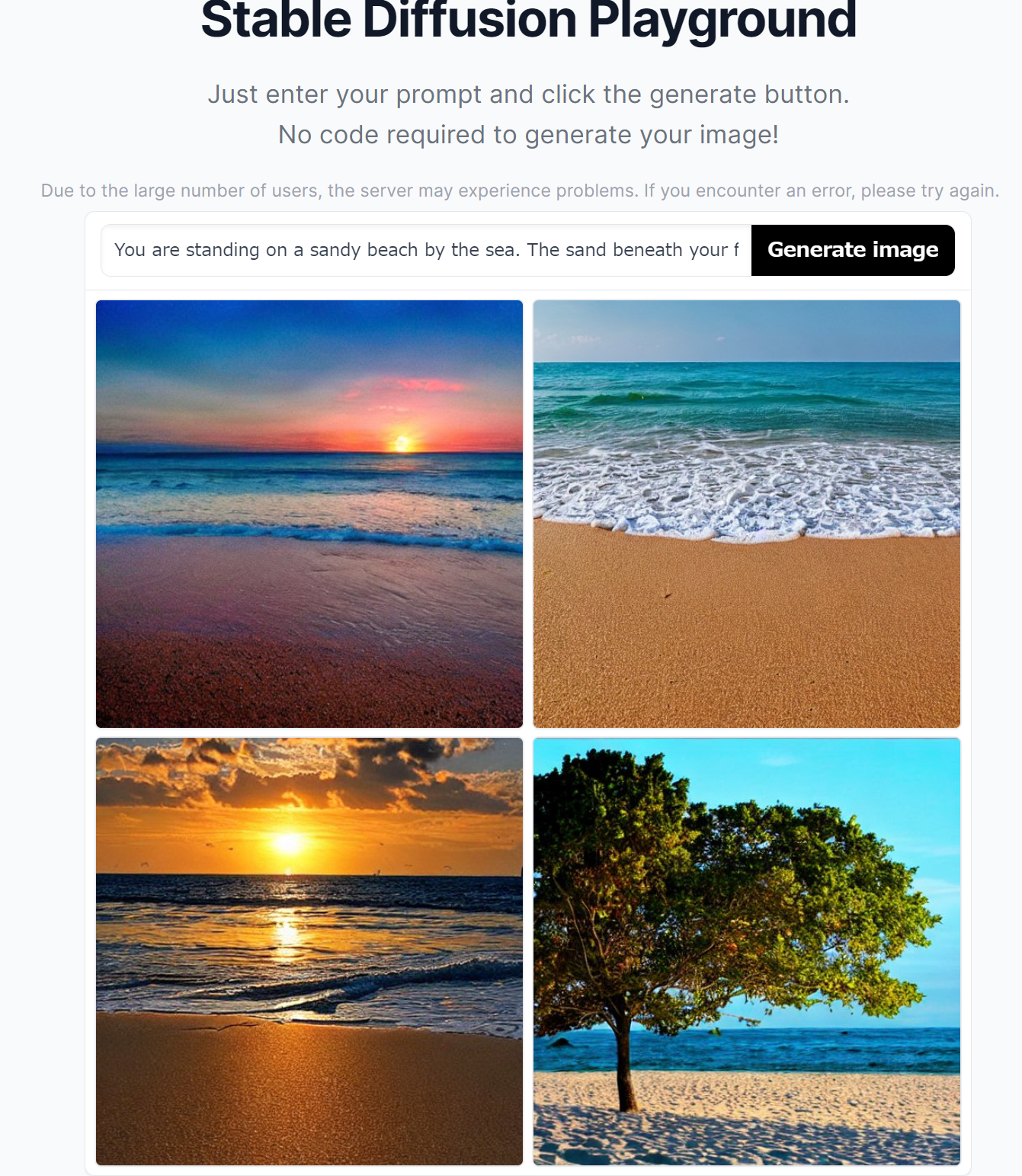
- Stable Diffusion 2-1 のページ(Hugging Face 上),オンラインデモ
https://huggingface.co/spaces/stabilityai/stable-diffusion
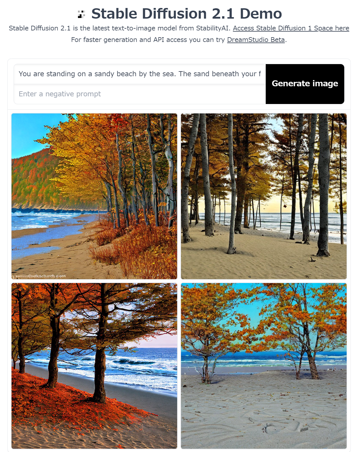
- stability-ai/stable-diffusion のページ(replicate 上),有料のサービス(登録を求められる)
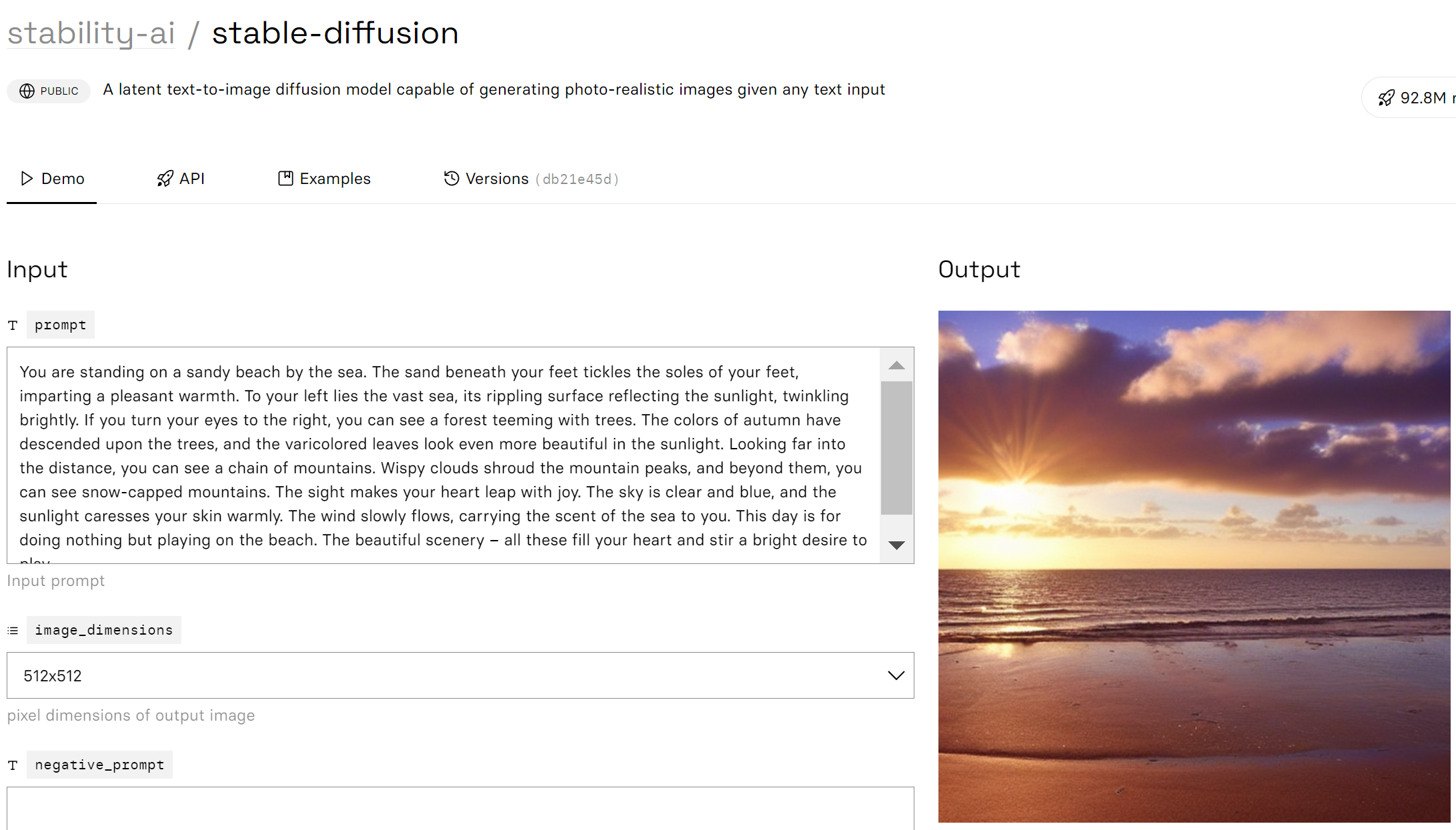
- cjwbw/anything-v4.0 のページ(replicate 上),有料のサービス(登録を求められる)
https://replicate.com/cjwbw/anything-v4.0
- cjwbw/anything-v3.0 のページ(replicate 上),有料のサービス(登録を求められる)
https://replicate.com/cjwbw/anything-v3.0
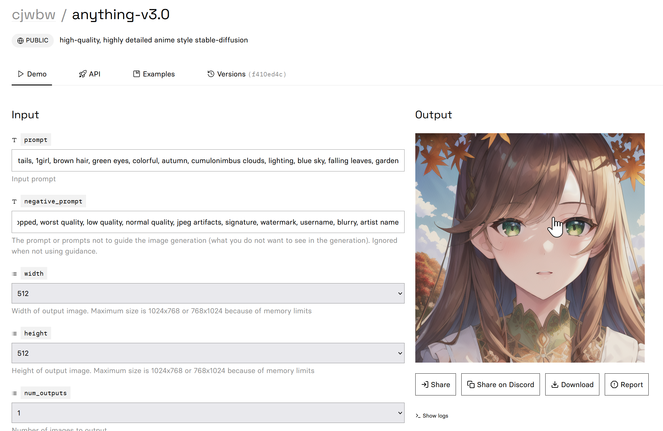
- cjwbw/waifu-diffusion のページ(replicate 上),有料のサービス(登録を求められる)
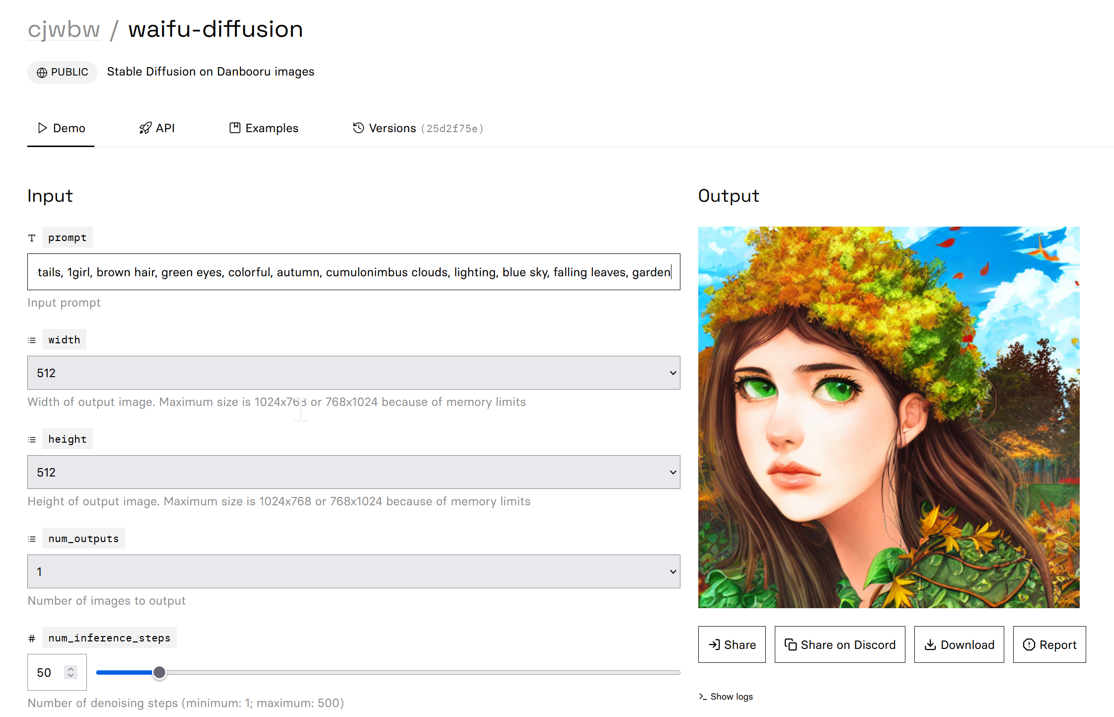
- Scribble Diffusion のページ,オンラインデモ
https://scribblediffusion.com/
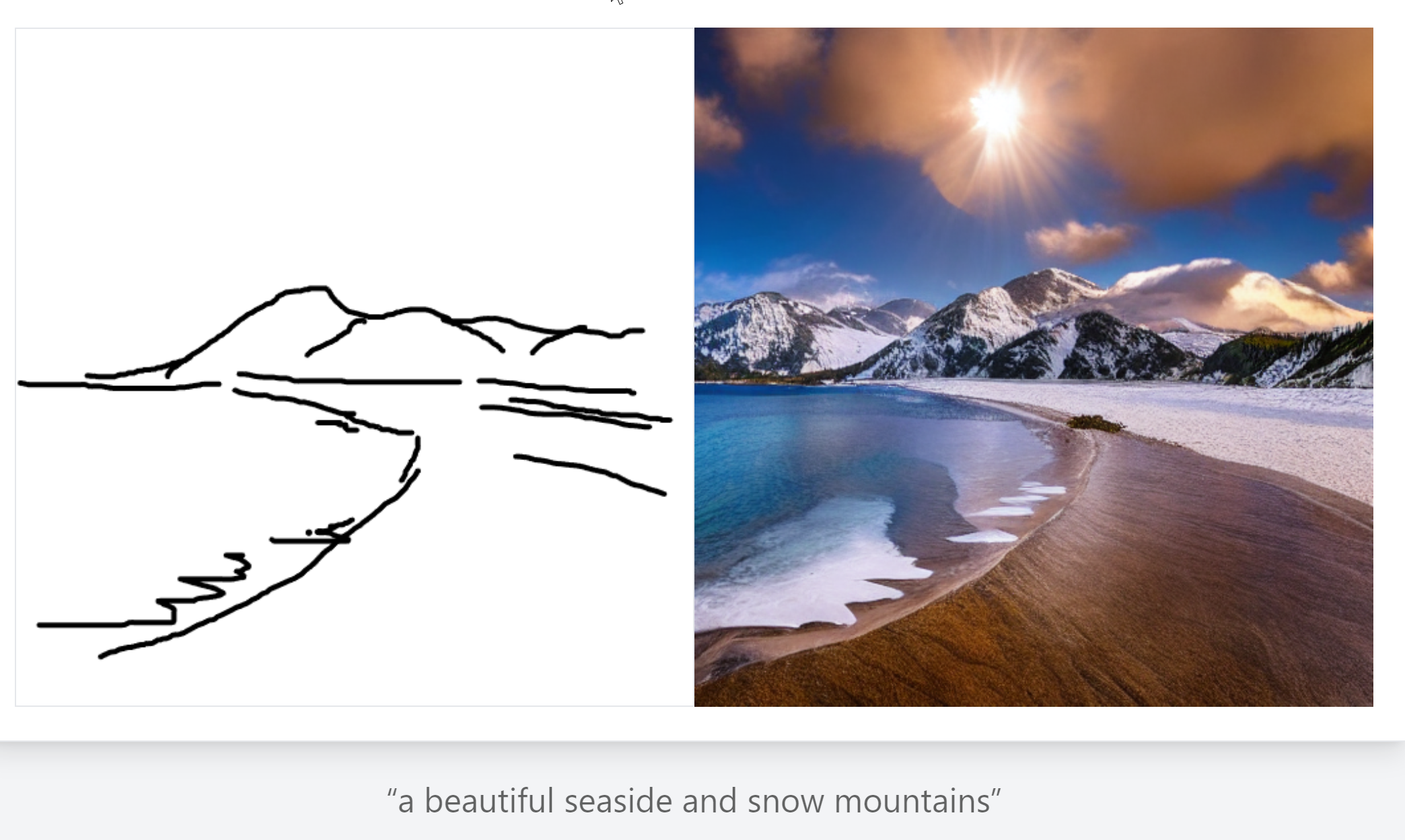
- andreasjansson/stable-diffusion-animation のページ (replicate 上),有料のサービス(登録を求められる)
https://replicate.com/andreasjansson/stable-diffusion-animation
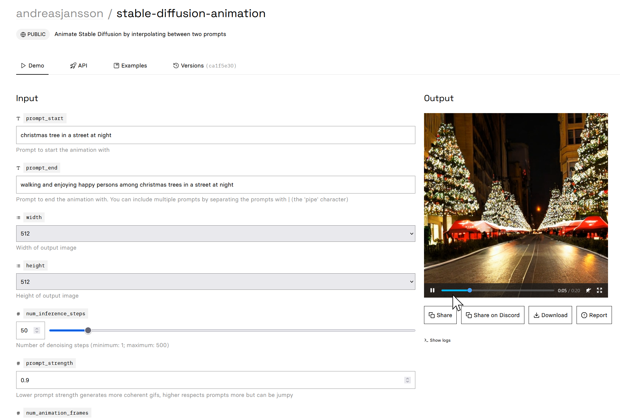
Stanford Alpaca
Stanford Alpaca は, スタンフォード大学で開発された 大規模言語モデルである. このモデルは,52Kの指示に準拠したLLaMA モデルの7Bデータセットをベースにしており,Self-Instruct によるファインチューニングを行っている.
Stanford Alpaca の生成手順は公開されており,さまざまなプロジェクトで利用されている.
【文献】
Rohan Taori and Ishaan Gulrajani and Tianyi Zhang and Yann Dubois and Xuechen Li and Carlos Guestrin and Percy Liang and Tatsunori B. Hashimoto, Stanford Alpaca: An Instruction-following LLaMA model, 2023.
【関連する外部ページ】
- Stanford Alpaca の GitHub のページ: https://github.com/tatsu-lab/stanford_alpaca
【関連項目】 LLaMA (Large Language Model Meta AI), Self-Instruct, 大規模言語モデル
short-time Fourier transform (STFT)
short-time Fourier transform (STFT) は, 短い区間のオーバーラッピングウインドウ (overlapping window) を 用いて離散フーリエ変換 (DFT) を行うことにより求める.
【関連項目】 librosa, 音データ(sound data)
SRCNN
SRCNN は,image super resolution の一手法.2015年発表.
Dong, Chao and Loy, Chen Change and He, Kaiming and Tang, Xiaoou, Image super-resolution using deep convolutional networks, IEEE transactions on pattern analysis and machine intelligence, vol. 38, no. 2, pp. 295--307, 2015.
【関連項目】 MMEditing, 超解像 (super resolution)
SSD
MMDetection に実装された SSD を用いた物体検出については,別項目で説明している.
- 文献
Liu, Wei and Anguelov, Dragomir and Erhan, Dumitru and Szegedy, Christian and Reed, Scott and Fu, Cheng-Yang and Berg, Alexander C., SSD: Single Shot MultiBox Detector, ECCV, also CoRR, https://arxiv.org/abs/1512.02325v5, 2016.
- 公式のソースコード (GitHub): https://github.com/weiliu89/caffe
- Papers with Code のページ: https://paperswithcode.com/paper/ssd-single-shot-multibox-detector
- MMDetection の SSD モデル: https://github.com/open-mmlab/mmdetection/blob/master/configs/ssd/README.md
【関連項目】 MMDetection, モデル, 物体検出
Structure from Motion (SfM)
SfM (Structure from Motion) は,オブジェクト(動かないもの)を, 周囲の複数の視点から撮影した多数の画像に対して次の処理を行う.
- それぞれの撮影での,視点の位置(3次元)と向きを推定する.
- 画像の特徴点について,位置(3次元)を推定する.
その結果,各画像の撮影位置と方向が推定されるとともに,オブジェクトの3次元点群が構成される.
SfM (Structure from Motion) の機能を持ったソフトウエアとしては, meshroom,OpenMVG などがある.
Ubuntu での OpenMVG のインストールは 別ページ »で説明
【関連項目】 3次元再構成 (3D reconstruction), meshroom, Multi View Stereo, OpenMVG, OpenMVS
SVHN (The Street View House Numbers) データセット
SVHN データセット は,公開されているデータセット(オープンデータ)である.
SVHN データセット は,小さく切り取られた数字の画像で,ラベル付けがされている. 機械学習での画像分類の学習や検証に利用できる.
- 実写(自然風景の画像中の数字や数値の認識)に由来.Google ストリートビュー画像中の家の番号から得ている.
- 0から9までの数字が示されたカラー画像.
- 数字が切り取られ,中央にくるように調整されているが,近くにある他の数字や,妨げになるようなものは,そのまま残されている.
- 画像の枚数:合計 630,420枚.
(内訳)
73,257枚:教師データ
26,032枚:検証データ
531,131枚:extra のデータ
- 画像のサイズ:32x32 である.
- RGB のカラー画像.
【文献】
Yuval Netzer, Tao Wang, Adam Coates, Alessandro Bissacco, Bo Wu, Andrew Y. Ng, Reading Digits in Natural Images with Unsupervised Feature Learning, NIPS Workshop on Deep Learning and Unsupervised Feature Learning 2011, 2011.
PDF ファイル:http://ufldl.stanford.edu/housenumbers/nips2011_housenumbers.pdf
【サイト内の関連ページ】
- SVHN データセットを扱う Python プログラム: 別ページ で説明している.
【関連する外部ページ】
- SVHN データセットの公式ページ: http://ufldl.stanford.edu/housenumbers/
- Papers With Code の SVHN データセットのページ: https://paperswithcode.com/dataset/svhn
- PyTorch の SVHN データセット: https://pytorch.org/vision/stable/datasets.html#torchvision.datasets.SVHN
- TensorFlow データセットの SVHN データセット: https://www.tensorflow.org/datasets/catalog/svhn_cropped
【関連項目】 TensorFlow データセット, オープンデータ, 画像分類
SwinIR
SwinIRは,超解像,ノイズ除去の一手法.
【文献】
Liang, Jingyun and Cao, Jiezhang and Sun, Guolei and Zhang, Kai and Van Gool, Luc and Timofte, Radu, SwinIR: Image Restoration Using Swin Transformer, arXiv preprint arXiv:2108.10257, 2021.
【関連する外部ページ】
GitHub のページ: https://github.com/JingyunLiang/SwinIR
TecoGAN
- 文献: Mengyu Chu, You Xie, Jonas Mayer, Laura Leal-Taixé, Nils Thuerey, Learning Temporal Coherence via Self-Supervision for GAN-based Video Generation, CoRR, abs/1811.09393v4, 2018.
- TecoGAN の GitHub のページ: https://github.com/thunil/TecoGAN
- 公式のデモページ(Google Colaboratory): https://colab.research.google.com/drive/1vgD2HML7Cea_z5c3kPBcsHUIxaEVDiIc
- Papers With Code のページ: https://paperswithcode.com/paper/temporally-coherent-gans-for-video-super
【関連項目】 GAN (Generative Adversarial Network), image super resolution, video super resolution
Temporal Segment Networks (TSN)
ビデオの動作認識 (action recognition) の一手法.2016年発表.
- 文献:
Wang, Limin and Xiong, Yuanjun and Wang, Zhe and Qiao, Yu and Lin, Dahua and Tang, Xiaoou and Van Gool, Luc, Temporal segment networks: Towards good practices for deep action recognition, European conference on computer vision, pp. 20--36, 2016.
- MMAction2 の Temporal Segment Networks (TSN) の説明ページ: https://github.com/open-mmlab/mmaction2/blob/master/configs/recognition/tsn/README.md
【関連項目】 MMAction2, 動作認識 (action recognition)
TensorFlow
TensorFlowは,Google が開発した機械学習フレームワークである.Python,C/C++言語から利用可能で,CPU,GPU,TPU 上で動作する.TensorFlowの特徴として「データフローグラフ」がある.これは,「データの流れ」を表現するもので,グラフの節点は演算(オペレーション)を,エッジはデータ(テンソル)の流れを表す.TensorFlowを使用することで,音声,画像,テキスト,ビデオなど多様なデータを扱う機械学習アプリケーションの開発が容易になる.2015年11月に初版がリリースされて以来,継続的にバージョンアップが続いている.
◯ TensorFlow GPU 版の動作に必要なもの
- 最新のNVIDIA ドライバ
Windows で,NVIDIA グラフィックス・ボードの種類を調べたいときは, hwinfo (URL: https://www.hwinfo.com/) を使って調べることができる.
- cudart64_110.dll, cusolver64_11.dll, cudnn64_8.dll など
そのために, 最新の NVIDIA cuDNNと, それに対応した,NVIDIA CUDA ツールキット 11を使う. (NVIDIA CUDA ツールキット は,バージョン12 でなくバージョン11 の最新版を使うこと.TensorFlow 2.10.1 で実際に試したが,バージョン 12 は不可)
最新の NVIDIA cuDNNに対応するNVIDIA CUDA ツールキットのバージョンは, NVIDIA cuDNN のページ https://developer.nvidia.com/cudnn で確認
- 古いバージョンである2.4.4 あるいはそれ以前のバージョンの TensorFlow を使う場合は, 最新の NVIDIA cuDNNを使わないこと. 詳しくは,別ページ »で説明
メッセージ
Internal: Attempting to perform BLAS operation using StreamExecutor without BLAS support
解決策:Python プログラムの先頭部分に次を追加すると解決する場合がある.
import tensorflow as tf
gpus = tf.config.list_physical_devices(device_type = 'GPU')
if len(gpus) > 0:
print("GPU:", gpus[0].name)
tf.config.experimental.set_memory_growth(gpus[0], True)
【文献】
TensorFlow: Large-Scale Machine Learning on Heterogeneous Distributed Systems
https://arxiv.org/pdf/1603.04467v2.pdf
【関連する外部ページ】
- TensorFlow の公式ページ: https://www.tensorflow.org
- Papers with Code のページ: https://paperswithcode.com/paper/tensorflow-large-scale-machine-learning-on
- GitHub のページ: https://github.com/tensorflow/tensorflow
- TensorFlow 2.0 リリースノート: https://github.com/tensorflow/tensorflow/releases/tag/v2.0.0
- チュートリアル: https://www.tensorflow.org/tutorials, https://github.com/nlintz/TensorFlow-Tutorials
- whitepaper: http://download.tensorflow.org/paper/whitepaper2015.pdf
【サイト内の関連ページ】
- GPU 環境でのTensorFlow 2.10.1 のインストールと活用(Windows 上): 別ページ »で説明
- Ubuntu での TensorFlow のインストール: 別ページ »で説明
【関連項目】 Applications of Deep Neural Networks, Keras, ディープラーニング
TensorFlow のレイヤ
TensorFlow のレイヤは,テンソルと設定オプションを入力とし,テンソルを出力とするような Python の関数である. TensorFlow を用いてニューラルネットワークを構築するときは, レイヤを組み立てていく. TensorFlow の Layers API は,以下のようなさまざまなタイプのレイヤを構築することができる.
- tf.layers.Dense: 全結合層
- tf.layers.Conv2D: 畳み込み層
TensorFlow の Layers API は,Keras の layers API の書き方に準拠している. TensorFlow の Layers API と Keras の layers API で関数名は同じである. 接頭語「tf.」の部分が異なる.
【関連項目】 TensorFlow
TensorFlow の Playground デモサイト
ニューラルネットワークのデモサイト: http://playground.tensorflow.org
【関連項目】 TensorFlow
TensorFlow Playground
TensorFlow Playground はオンラインで動く. ニューラルネットワークの ニューロン,結合,学習,重みの変化,学習率,活性化関数(ReLU など),正則化(L2 正則化など),バッチサイズ,データの分類,回帰,そして,ハイパーパラメータが,学習にどのように影響するかなどを簡単に確認できるオンラインのサービスである. URL は次の通り.
http://playground.tensorflow.org
【関連項目】 TensorFlow
TensorFlow-Slim
TensorFlow-Slimは,CNN (convolutional neural network) による画像分類のモデルで利用される学習や検証の機能を持つ. 微調整 (fine tuning)の機能も持つ.
TensorFlow-Slimは,TensorFlow 1.14 から 2.2 で動くようである (根拠: https://github.com/google-research/tf-slim). 最新の TensorFlow で動くとは限らないので,利用者で確認すること.
- 出典
N. Silberman and S. Guadarrama, TensorFlow-Slim image classification model library, 2016.
- URL: https://github.com/tensorflow/models/tree/master/research/slim
【関連項目】 TensorFlow のモデルガーデン, TensorFlow
TensorFlow データセット
TensorFlow データセットのカタログのページ: https://www.tensorflow.org/datasets/catalog/overview
「tfds.list_builders()」により,現在インストールされている TensorFlow データセットの データセットビルダーを確認できる.
TensorFlow データセットのロード時に分割を行うには,次のように書く.
「0%:50%」は先頭から 50 %, 「50%:100%」は末尾の 50% 部分.
from __future__ import absolute_import, division, print_function, unicode_literals
import tensorflow as tf
import numpy as np
import tensorflow_datasets as tfds
%matplotlib inline
import matplotlib.pyplot as plt
import warnings
warnings.filterwarnings('ignore') # Suppress Matplotlib warnings
iris, iris_info = tfds.load('iris', split=['train[0%:50%]', 'train[50%:100%]'], with_info = True, shuffle_files=True, as_supervised=True)
iris = {'train': iris[0], 'test': iris[1]}
【関連項目】 CIFAR-10 データセット, CIFAR-100 データセット, Fashion MNIST データセット, IMDb データセット, MNIST データセット, くずし字 MNIST データセット(Kuzushiji-MNIST データセット), TensorFlow
TensorFlow データセットカタログ
TensorFlow データセットカタログ の URL: https://www.tensorflow.org/datasets/catalog/overview
【関連項目】 TensorFlow
TensorFlow のモデルガーデン
URL: https://github.com/tensorflow/models
Windows では,次のような手順でダウンロードできる.
「c:\Program Files\Python38」のところは,Python のインストールディレクトリを設定すること.
- Git のインストール: 別項目で説明している.
Git の公式ページ: https://git-scm.com/
- ダウンロード
cd "c:\Program Files\Python38\Lib" git clone --recursive https://github.com/tensorflow/models -
必要に応じて,次のようなコマンドで,シンボリックリンクを作っておくと便利である.
cd "c:\Program Files\Python38\Lib" mklink /D slim models\research\slim
【関連項目】 TensorFlow-Slim, TensorFlow
Tensorpack
Saliency Map
!pip3 install --upgrade git+https://github.com/tensorpack/tensorpack.git
%tensorflow_version 1.x
%cd /content
!rm -rf tensorpack
!git clone https://github.com/tensorpack/tensorpack
%cd tensorpack
%cd examples/Saliency
!curl -O http://download.tensorflow.org/models/resnet_v1_50_2016_08_28.tar.gz
!tar -xzvf resnet_v1_50_2016_08_28.tar.gz
!curl -L https://github.com/opencv/opencv/blob/master/samples/data/squirrel_cls.jpg?raw=true -o squirrel_cls.jpg
!python3 ./saliency-maps.py squirrel_cls.jpg
Tesseract OCR
Tesseract OCR は,文字認識ソフトウェアである.
【サイト内の関連ページ】
- Tesseract OCR の使い方: 別ページ »にまとめ
- Windows での Tesseract OCR 5.3.3 のインストールと動作確認(多言語の文字認識): 別ページ »で説明
- Ubuntu での Tesseract OCR のインストール: 別ページ »で説明
【関連する外部ページ】
GitHub の Tesseract OCR のページ: https://github.com/tesseract-ocr/tesseract
Theano
(2017年9月に開発の停止がアナウンスされた)
- GitHub の公式ページ: https://github.com/Theano/
- チュートリアル: https://github.com/Newmu/Theano-Tutorials
- CoRR, abs/1605.02688
- Wikipedia のページ: https://en.wikipedia.org/wiki/Theano_(software)
TinaFace
TinaFace は顔検出法である. ResNet50 と Feature Pyramid Network (FPN) をベースとする顔検出法. FPN は 6 レベルあり,それを踏襲している. そうした仕組みになっていることから,さまざまなサイズの顔を検出できるとされている. WIDER FACE データセットを用いた検証により,当時の他の顔検出法よりも精度が優れているとされている.
- 文献
Yanjia Zhu, Hongxiang Cai, Shuhan Zhang, Chenhao Wang, Yichao Xiong, TinaFace: Strong but Simple Baseline for Face Detection, 2020, arXiv:2011.13183 [cs.CV],
- ResearchGate のページ: https://www.researchgate.net/publication/346475155_TinaFace_Strong_but_Simple_Baseline_for_Face_Detection
- Papers with Code のページ: https://paperswithcode.com/method/tinaface
【関連項目】 RetinaNet, SCRFD, モデル, 顔検出 (face detection)
Titanic データセット
Titanic データセットは,公開されているデータセット(オープンデータ)である.
- 行数: 1309行
- 属性: pclass, name, sex, age, sibsp, parch, ticket, fare, cabin, embarked, boat, body, home.dest, survived
【文献】
Frank E. Harrell Jr., Thomas Cason, Titanic dataset, 2002.
【サイト内の関連ページ】
- Titanic データセットについての説明資料: titanic.pdf [PDF], [パワーポイント]
- Titanic データセットを扱う Python プログラム: 別ページ で説明している.
【関連する外部ページ】
- TensorFlow データセットの titanic データセット: https://www.tensorflow.org/datasets/catalog/titanic
Transformers
【関連項目】 GPT-2, text generation, テキスト特徴 (text feature)
t 検定 (t test)
- 正規分布に従う2群について,等分散性が成り立っていることが確実な場合には var.equal=TRUE を指定する.
- 正規分布に従う2群について,等分散性が成り立っていない可能性がある場合には, var.equal=FALSE を指定する.(等分散性を仮定しない t 検定を, ウェルチの検定ともいう)
t.test(s1, s2, var.equal=TRUE)
t.test(s1, s2, var.equal=FALSE)
【関連項目】 検定
U2-Net
U2-Net は salient object detection の一手法.
【文献】
Xuebin Qin, Zichen Zhang, Chenyang Huang, Masood Dehghan, Osmar R. Zaiane and Martin Jagersand, U2-Net: Going Deeper with Nested U-Structure for Salient Object Detection, arXiv:2005.09007, 2020.
【サイト内の関連ページ】
rembg のインストールと動作確認(画像の背景除去)(Python を使用)(Windows 上): 別ページ »で説明
【関連する外部ページ】
- 公式の GitHub のページ: https://github.com/xuebinqin/U-2-Net
- Papers With Code のページ: https://paperswithcode.com/method/u2-net
【関連項目】 BASNet, U-Net, salient object detection, セマンティック・セグメンテーション (semantic segmentation)
UCF101 (UCF101 Human Actions dataset)
ビデオでのアクションの認識. UCF101 データセット は,101 のアクションカテゴリに分類済みの動画のデータセットである.
- YouTube から収集された 13,320個の動画
- 101のアクションカテゴリに分類済み,5つのタイプ(体の動き,人と人のインタラクション,人とモノのインタラクション,楽器演奏,スポーツ)に大別される.
- フレームレートは 25FPS,解像度は 320x240.
UCF101 データセットは次の URL で公開されているデータセット(オープンデータ)である.
https://www.crcv.ucf.edu/data/UCF101.php
【関連情報】
- UCF101: A Dataset of 101 Human Actions Classes From Videos in The Wild, Khurram Soomro, Amir Roshan Zamir, Mubarak Shah
- Papers With Code の UCF101 データセットのページ: https://paperswithcode.com/dataset/ucf101
- PyTorch の UCF101 データセット: https://pytorch.org/vision/stable/datasets.html#torchvision.datasets.UCF101
- TensorFlow データセットの UCF101 データセット: https://www.tensorflow.org/datasets/catalog/ucf101
UCF-QNRF データセット
画像数は 1,535枚. 各画像のアノテーションされたオブジェクト数は 49 から 12,865 である.
- 文献
Haroon Idrees, Muhmmad Tayyab, Kishan Athrey, Dong Zhang, Somaya Al-Maadeed, Nasir Rajpoot, and Mubarak Shah. Composition loss for counting, density map estimation and localization in dense crowds. In ECCV, 2018.
- 公式ページ: https://www.crcv.ucf.edu/data/ucf-qnrf/
【関連項目】 crowd counting, FIDTM, オープンデータ
U-Net
- 文献
Olaf Ronneberger, Philipp Fischer, Thomas Brox, U-Net: Convolutional Networks for Biomedical Image Segmentation, CoRR, abs/1505.04597v1, 2015.
- U-Net のページ
https://lmb.informatik.uni-freiburg.de/people/ronneber/u-net/
- 実装されたソースコード等 (GitHub) のページ: https://github.com/milesial/PyTorch-UNet
【関連項目】 BASNet, セマンティック・セグメンテーション (semantic segmentation), salient object detection
Unified Scene Text Detection
Unified Scene Text Detection は,テキスト検出(text detection),ドキュメントのレイアウト解析(layout analysis)を統合することにより,精度の改善を行っている. 2022年発表.
【文献】
Towards End-to-End Unified Scene Text Detection and Layout Analysis, Long, Shangbang and Qin, Siyang and Panteleev, Dmitry and Bissacco, Alessandro and Fujii, Yasuhisa and Raptis, Michalis, Proceedings of the IEEE/CVF Conference on Computer Vision and Pattern Recognition, 2022.
https://arxiv.org/abs/2203.15143
【サイト内の関連ページ】
Unified Scene Text Detection のインストールとテスト実行(テキスト検出)(Python,TensorFlow を使用)(Windows 上): 別ページ »で説明
【関連する外部ページ】
- Unified Scene Text Detection の GitHub の公式ページ: https://github.com/tensorflow/models/tree/master/official/projects/unified_detector
- Papers With Code のページ: https://paperswithcode.com/paper/towards-end-to-end-unified-scene-text
【関連項目】 HierText
UTKFace データセット
20,000枚以上の顔画像,68ランドマーク,各種の属性(年齢,性別など)を含む.
次の URL で公開されているデータセット(オープンデータ)である.
UTKFace の URL: https://susanqq.github.io/UTKFace/
【関連項目】 顔のデータベース, 顔ランドマーク (facial landmark)
VALL-E X
VALL-E X は,音声合成(TTS),プロンプトとして音声を与えて音声合成(voice cloning)の技術である.
【サイト内の関連ページ】
- VALL-E X のインストールと動作確認(音声合成)(Python を使用)(Windows 上): 別ページ »で説明
【関連する外部ページ】
- Plachtaa/VALL-E-X の実装の GitHub のページ: https://github.com/Plachtaa/VALL-E-X
- Plachtaa/VALL-E-X の実装の Hugging Face のデモページ: https://huggingface.co/spaces/Plachta/VALL-E-X
【関連項目】 Bark
VGGFace2 データセット
VGGFace2 データセットは,顔画像がクラス分けされたデータセットである.
- 画像は,約331万枚.訓練用と検証用に分かれ,うち検証用は約17万枚である.
- クラスは,9,131 クラス.訓練用の画像は,8,631クラスに分かれている.
- 平均解像度は 137x180 画素.32 画素以下の解像度のものは,全体の 1%未満である.
作者からは,社会的,性別的,人種的,その他の偏りに注意して使うように,注意が行われている.
次の URL で公開されているデータセット(オープンデータ)である.
https://www.robots.ox.ac.uk/~vgg/data/vgg_face/
- Qiong Cao, Li Shen, Weidi Xie, Omkar M. Parkhi, Andrew Zisserman, VGGFace2: A dataset for recognising faces across pose and age, 2018 13th IEEE International Conference on Automatic Face & Gesture Recognition, vol. 1, pages: 66-74, 2018.
- Papers With Code の VGGFace2 データセットのページ: https://paperswithcode.com/dataset/vggface2-1
【関連項目】 facial inpainting, 顔のデータベース, 顔認識
Vision Transformer
Vision Transformer は, 画像分類を,CNN よりも高速に,CNN よりも精度が落ちることなく実行できるとされる.
- 文献
Alexey Dosovitskiy, Lucas Beyer, Alexander Kolesnikov, Dirk Weissenborn, Xiaohua Zhai, Thomas Unterthiner, Mostafa Dehghani, Matthias Minderer, Georg Heigold, Sylvain Gelly, Jakob Uszkoreit, Neil Houlsby, An Image is Worth 16x16 Words: Transformers for Image Recognition at Scale, ICLR 2021, 2021.
【関連する外部ページ】
- Google Colab デモ: https://colab.research.google.com/github/google-research/vision_transformer/blob/master/vit_jax.ipynb
- Google Colab デモ(AugReg): https://colab.research.google.com/github/google-research/vision_transformer/blob/master/vit_jax_augreg.ipynb
- 非公式の PyTorch での ViT の実装: https://github.com/lucidrains/vit-pytorch
【関連項目】 画像分類
VOICEVOX
VOICEVOX は,音声合成のソフトウェアである.
VOICEVOX CORE の GitHub のページ: https://github.com/VOICEVOX/voicevox_core
【関連項目】 音声合成 (Text To Speech; TTS)
Wasserstein GAN (WGAN)
Wasserstein GANでは, GAN (Generative Adversarial Network) での勾配消失問題の解決に取り組んでいる. GAN (Generative Adversarial Network) で用いられてきた Jensen-Shannon divergence(確率密度間の距離尺度の1つ) の代わりに Wasserstein 距離を用いる. 安定して学習ができるとされている.
- 文献:
Martin Arjovsky, Soumith Chintala, Léon Bottou, Wasserstein GAN, 2017.
CoRR, abs/1701.07875v3
- Papers with Code のページ: https://paperswithcode.com/method/wgan
- PyTorch-GAN のページ: https://github.com/eriklindernoren/PyTorch-GAN
- Keras-GAN のページ: https://github.com/eriklindernoren/Keras-GAN
- labmlai/annotated_deep_learning_paper_implementations のページ: https://github.com/labmlai/annotated_deep_learning_paper_implementations
【関連項目】 GAN (Generative Adversarial Networks), image generation
Wasserstein GAN with Gradient Penalty (WGAN-GP)
- 文献: Ishaan Gulrajani, Faruk Ahmed, Martin Arjovsky, Vincent Dumoulin, Aaron Courville, Improved Training of Wasserstein GANs, NeurIPS 2017, 2017.
- Papers with Code のページ: https://paperswithcode.com/paper/improved-training-of-wasserstein-gans
- PyTorch-GAN のページ: https://github.com/eriklindernoren/PyTorch-GAN
- Keras-GAN のページ: https://github.com/eriklindernoren/Keras-GAN
- labmlai/annotated_deep_learning_paper_implementations のページ: https://github.com/labmlai/annotated_deep_learning_paper_implementations
【関連項目】 GAN (Generative Adversarial Networks), image generation, Wasserstein GAN (WGAN)
WebFace260M, WebFace42M データセット
機械学習向けの大規模な顔画像のデータセット. 顔検出,顔の分類(年齢,性別など)の用途が想定されている.2021年時点では,研究者等が利用可能な,最大規模の顔画像のデータセットである. データは次の2種類がある.
- WebFace260M:
4M identities, 260M images, images/id 64, cleaning no, public
- WebFace42M
2M identities, 42M images, images/id 21, cleaning auto, 7 attributes 訓練データに適するとされている.年齢,人種,性別,シナリオ(controlled, in-the-wild, cross-scene)
次の URL で公開されているデータセット(オープンデータ)である.
URL: https://www.face-benchmark.org/index.html
詳細は,「the Masked Face Recognition challenge」の文献で説明されている.
- Papers with Code のページ: https://paperswithcode.com/dataset/webface260m
- 文献
Zheng Zhu, Guan Huang, Jiankang Deng, Yun Ye, Junjie Huang, Xinze Chen, Jiagang Zhu, Tian Yang, Jiwen Lu, Dalong Du, Jie Zhou, WebFace260M: A Benchmark Unveiling the Power of Million-scale Deep Face Recognition, IEEE Conference on Computer Vision and Pattern Recognition (CVPR), 2021
- 文献
Zheng Zhu, Guan Huang, Jiankang Deng, Yun Ye, Junjie Huang, Xinze Chen, Jiagang Zhu, Tian Yang, Jia Guo, Jiwen Lu, Dalong Du, and Jie Zhou. Masked face recognition challenge: The WebFace260M track report. arXiv:2108.07189, 2021.
【関連項目】 顔のデータベース
Whisper
Whisperは,音声からの文字起こし,翻訳を行う. 訓練されたモデルが既存のデータセットにゼロショットで適用可能であり,データセット固有のファインチューニングを必要とせずに高品質な結果を達成することを特徴とする.
【文献】
Alec Radford, Jong Wook Kim, Tao Xu, Greg Brockman, Christine McLeavey, Ilya Sutskever, Robust Speech Recognition via Large-Scale Weak Supervision, CoRR abs/2212.04356, 2022.
https://cdn.openai.com/papers/whisper.pdf
【サイト内の関連ページ】
- マイクに話しかけた言葉を,リアルタイムにAIが認識(whisper, whisper_mic, Python を使用)(Windows 上)別ページ »で説明
- Whisper のインストール,Whisper を使う Python プログラム(音声からの文字起こし,翻訳)(Python,PyTorch を使用)(Windows 上)別ページ »で説明
【関連する外部ページ】
- Papers with Code のページ: https://paperswithcode.com/paper/robust-speech-recognition-via-large-scale-1
- Introducing Whisper のページ: https://openai.com/index/whisper/
- GitHub のページ: https://github.com/openai/whisper
【関連項目】 mallorbc の whisper_mic
Wide ResNet
【関連項目】 Residual Networks (ResNets), モデル, 画像分類
PyTorch, torchvision の Wide ResNet50 学習済みモデルのロード,画像分類のテスト実行
Google Colab あるいはパソコン(Windows あるいは Linux)を使用.
- 前準備
前準備として,Python のインストール: 別項目で説明している. PyTorch のインストール を行う.
Google Colaboratory では, Python, PyTorch はインストール済みなので,インストール操作は不要.次に,pip を用いて,pillow のインストールを行う.
pip install -U pillow - ImageNet データセット で学習済みのWide ResNet モデルのロード
PyTorch, torchvision のモデルについては: https://pytorch.org/vision/stable/models.html に説明がある.
import torch import torchvision.models as models device = torch.device('cuda' if torch.cuda.is_available() else 'cpu') m = models.wide_resnet50_2(pretrained=True).to(device) - 画像分類したい画像ファイルのダウンロードとロードと確認表示
from PIL import Image
import requests
from IPython.display import display

# ダウンロードとロード
url = 'https://github.com/pytorch/hub/raw/master/images/dog.jpg'
response = requests.get(url)
img = Image.open(requests.get(url, stream=True).raw)

# 確認表示
display(img)
- 画像の前処理.PyTorch で扱えるようにするため.
from PIL import Image from torchvision import transforms img = Image.open(filename) preprocess = transforms.Compose([ transforms.Resize(256), transforms.CenterCrop(224), transforms.ToTensor(), transforms.Normalize(mean=[0.485, 0.456, 0.406], std=[0.229, 0.224, 0.225]), ]) input_tensor = preprocess(img) input_batch = input_tensor.unsqueeze(0) - 推論 (inference) の実行
「m.eval()」は,推論を行うときのためのもの.これを行わないと訓練(学習)が行われる.
import torch if torch.cuda.is_available(): input_batch = input_batch.to('cuda') m.eval() with torch.no_grad(): output = m(input_batch) - 結果の表示
import urllib
url, filename = ("https://raw.githubusercontent.com/pytorch/hub/master/imagenet_classes.txt", "imagenet_classes.txt")
try: urllib.URLopener().retrieve(url, filename)
except: urllib.request.urlretrieve(url, filename)

with open("imagenet_classes.txt", "r") as f:
    categories = [s.strip() for s in f.readlines()]

# The output has unnormalized scores. To get probabilities, you can run a softmax on it.
probabilities = torch.nn.functional.softmax(output[0], dim=0)
print(probabilities)

top5_prob, top5_catid = torch.topk(probabilities, 5)
for i in range(top5_prob.size(0)):
    print(categories[top5_catid[i]], top5_prob[i].item())
Google Colaboratory での結果
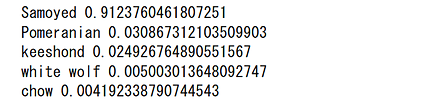
Windows での結果
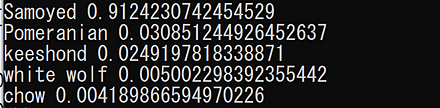
Linux での結果
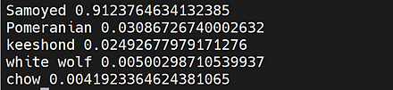
PyTorch, torchvision の Wide ResNet101 学習済みモデルのロード,画像分類のテスト実行
Google Colab あるいはパソコン(Windows あるいは Linux)を使用.
- 前準備
前準備として,Python のインストール: 別項目で説明している. PyTorch のインストール を行う.
Google Colaboratory では, Python, PyTorch はインストール済みなので,インストール操作は不要.次に,pip を用いて,pillow のインストールを行う.
pip install -U pillow - ImageNet データセット で学習済みのWide ResNet モデルのロード
PyTorch, torchvision のモデルについては: https://pytorch.org/vision/stable/models.html に説明がある.
import torch import torchvision.models as models device = torch.device('cuda' if torch.cuda.is_available() else 'cpu') m = models.wide_resnet101_2(pretrained=True).to(device) - 画像分類したい画像ファイルのダウンロードとロードと確認表示
from PIL import Image
import requests
from IPython.display import display

# ダウンロードとロード
url = 'https://github.com/pytorch/hub/raw/master/images/dog.jpg'
response = requests.get(url)
img = Image.open(requests.get(url, stream=True).raw)

# 確認表示
display(img)
- 画像の前処理.PyTorch で扱えるようにするため.
from PIL import Image from torchvision import transforms img = Image.open(filename) preprocess = transforms.Compose([ transforms.Resize(256), transforms.CenterCrop(224), transforms.ToTensor(), transforms.Normalize(mean=[0.485, 0.456, 0.406], std=[0.229, 0.224, 0.225]), ]) input_tensor = preprocess(img) input_batch = input_tensor.unsqueeze(0) - 推論 (inference) の実行
「m.eval()」は,推論を行うときのためのもの.これを行わないと訓練(学習)が行われる.
import torch if torch.cuda.is_available(): input_batch = input_batch.to('cuda') m.eval() with torch.no_grad(): output = m(input_batch) - 結果の表示
import urllib
url, filename = ("https://raw.githubusercontent.com/pytorch/hub/master/imagenet_classes.txt", "imagenet_classes.txt")
try: urllib.URLopener().retrieve(url, filename)
except: urllib.request.urlretrieve(url, filename)

with open("imagenet_classes.txt", "r") as f:
    categories = [s.strip() for s in f.readlines()]

# The output has unnormalized scores. To get probabilities, you can run a softmax on it.
probabilities = torch.nn.functional.softmax(output[0], dim=0)
print(probabilities)

top5_prob, top5_catid = torch.topk(probabilities, 5)
for i in range(top5_prob.size(0)):
    print(categories[top5_catid[i]], top5_prob[i].item())
Google Colaboratory での結果
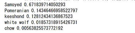
Windows での結果
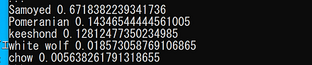
Linux での結果
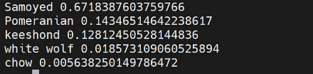
WIDER FACE データセット
WIDER FACE データセットは,32,203枚の顔画像のデータセットである. 機械学習での顔検出の学習や検証に利用できる.
- 公開されている WIDERデータセットから,32,203枚の画像が選択された.
- その中の 393,703個の顔について,バウンディングボックスが付けられている.
- 顔のサイズ,ポーズ,occlusion,表情,照明,イベントはさまざまである.
- 61のシーンカテゴリ(scene category)が定められている.各シーンカテゴリについて,40%/10%/50%の比率で,画像がランダムに選択され,訓練データ(training data),検証データ(validation data),テストデータ(test data)に分けられている.
- EdgeBoxes 法による検出率により,Easy, Medium, Hard の 3つの困難さのレベルが定められている.
- 訓練データと検証データの画像とアノテーションはオンラインで公開されているが,テストデータのアノテーションは公開されていない(結果はデータベースサーバーに送られ,精度とリコール曲線を受け取ることになっている).
WIDER FACE データセットは,次の URL で公開されているデータセット(オープンデータ)である.
URL: http://shuoyang1213.me/WIDERFACE/
【関連情報】
- Yang, Shuo and Luo, Ping and Loy, Chen Change and Tang, Xiaoou, WIDER FACE: A Face Detection Benchmark, IEEE Conference on Computer Vision and Pattern Recognition (CVPR),2016.
- PyTorch の WIDER FACE データセット: https://pytorch.org/vision/stable/datasets.html
- TensorFlow データセットの WIDER FACE データセット: https://www.tensorflow.org/datasets/catalog/wider_face
【関連項目】 顔のデータベース, 顔検出 (face detection)
YOLOv3
- 文献
Redmon, Joseph and Farhadi, Ali, YOLOv3: An Incremental Improvement, CoRR, abs/1804.02767v1, 2018.
- Papers with Code のページ: https://paperswithcode.com/paper/yolov3-an-incremental-improvement
- AlexeyAB darknet: https://github.com/AlexeyAB/darknet
- AlexeyAB darknet のアセット: https://github.com/AlexeyAB/darknet/releases/
- MMDetection のモデル: https://github.com/open-mmlab/mmdetection/blob/master/configs/yolo/README.md
- MMDetection: https://github.com/open-mmlab/mmdetection
【関連項目】 AlexeyAB darknet, MMDetection, YOLOv4, YOLOX, モデル, 物体検出
Google Colaboratory で YOLOv3 による物体検出(AlexeyAB darknet を使用)
次のコマンドやプログラムは Google Colaboratory で動く(コードセルを作り,実行する)
- Google Colaboratory で,ランタイムのタイプを GPU に設定する.
- AlexeyAB darknet のビルド
%cd /content
!rm -rf darknet
!git clone https://github.com/AlexeyAB/darknet
%cd darknet
!make GPU=1 CUDNN=1 CUDNN_HALF=1 OPENCV=1
- 重みのダウンロード
AlexeyAB darknet のアセット: https://github.com/AlexeyAB/darknet/releases/
!curl -LO https://github.com/AlexeyAB/darknet/releases/download/darknet_yolo_v3_optimal/yolov3.weights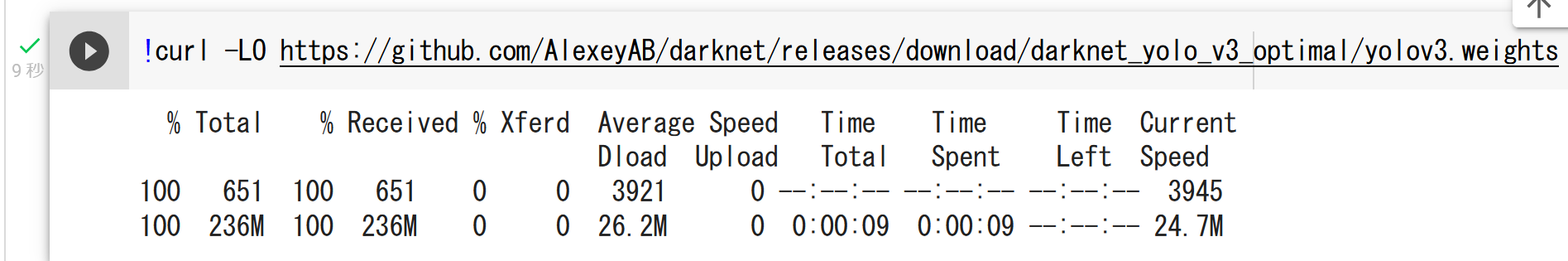
- YOLOv3 による物体検出
!rm -r predictions.jpg
!./darknet detector test cfg/coco.data cfg/yolov3.cfg yolov3.weights data/dog.jpg -dont_show
from PIL import Image
Image.open('predictions.jpg').show()
!./darknet detector test cfg/coco.data cfg/yolov3.cfg yolov3.weights data/giraffe.jpg -dont_show
Image.open('predictions.jpg').show()
!./darknet detector test cfg/coco.data cfg/yolov3.cfg yolov3.weights data/horses.jpg -dont_show
Image.open('predictions.jpg').show()
!./darknet detector test cfg/coco.data cfg/yolov3.cfg yolov3.weights data/person.jpg -dont_show
Image.open('predictions.jpg').show()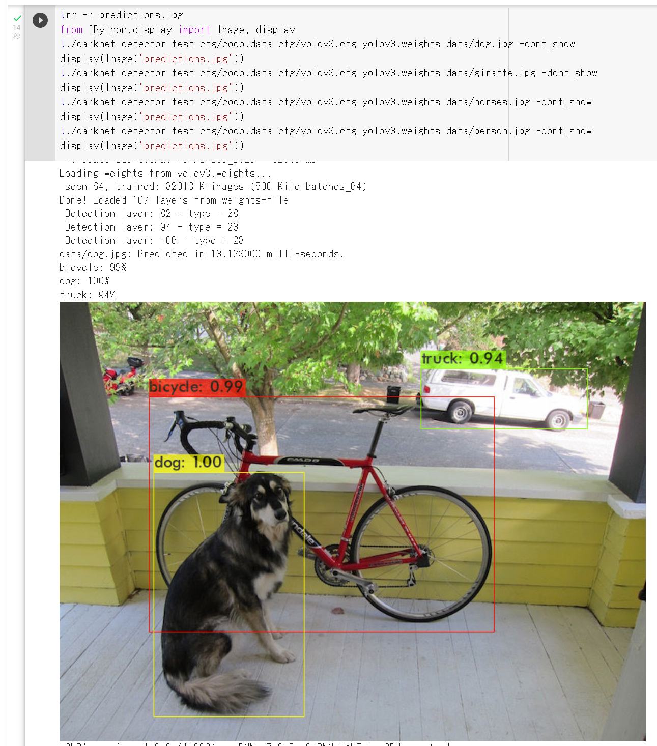
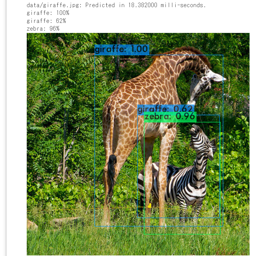
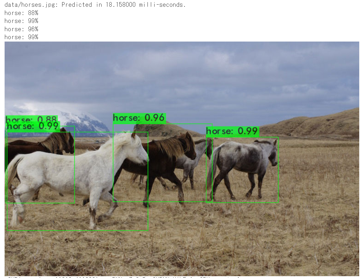
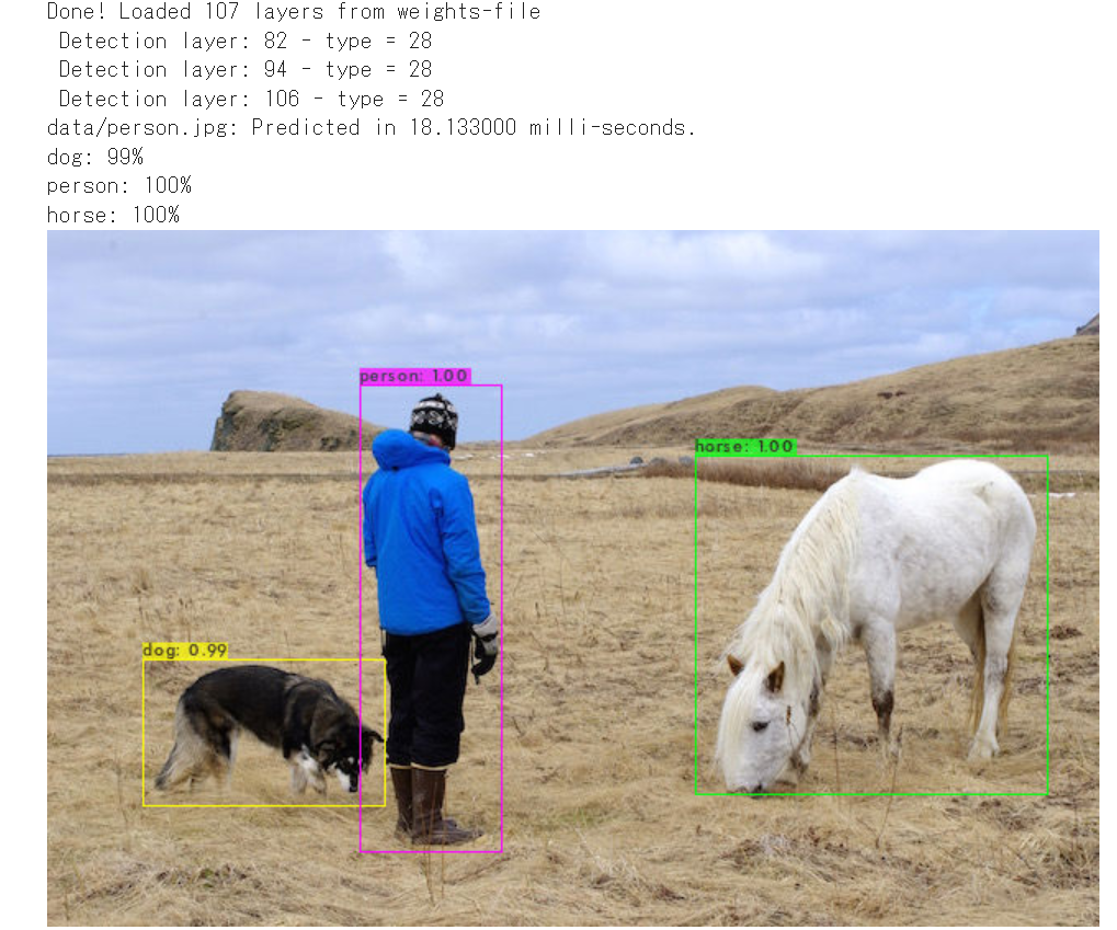
Google Colaboratory で AlexeyAB darknet のインストールと,YOLOv3 による物体検出(AlexeyAB darknet を使用)
書きかけ(動作チェック中)
cd %LOCALAPPDATA%
rmdir /s /q darknet
git clone https://github.com/AlexeyAB/darknet
cd darknet
del CMakeCache.txt
rmdir /s /q CMakeFiles
cmake -A x64 -T host=x64 ^
    -DCUDA_BUILD_CUBIN=ON -DENABLE_CUDA=ON -DENABLE_CUDNN=ON -DENABLE_CUDNN_HALF=ON
cmake --build . --config Release --target INSTALL -- /m:4

 Windows では,システム環境変数 PATH に,次の2つを追加.

    %LOCALAPPDATA%\darknet\build\darknet\x64
    %LOCALAPPDATA%\darknet\3rdparty\pthreads\bin

cd %LOCALAPPDATA%
cd darknet
curl -LO https://github.com/AlexeyAB/darknet/releases/download/darknet_yolo_v3_optimal/yolov3.weights
darknet detect cfg/yolov3.cfg yolov3.weights data/dog.jpg -ext_output
darknet detect cfg/yolov3.cfg yolov3.weights data/giraffe.jpg -ext_output
darknet detect cfg/yolov3.cfg yolov3.weights data/horses.jpg -ext_output
darknet detect cfg/yolov3.cfg yolov3.weights data/person.jpg -ext_output
curl -O https://www.kkaneko.jp/sample/video/samplevideo.mp4
./darknet detector demo cfg/coco.data cfg/yolov3.cfg yolov3.weights samplevideo.mp4 -i 0 -thresh 0.25
Avatar Erik Linder-Norén による YOLOv3 の実装の,Ubuntu でのインストールと実行
Avatar Erik Linder-Norén による YOLOv3 の実装: https://github.com/eriklindernoren/PyTorch-YOLOv3
- インストールとテスト実行
Ubuntu では,次のコマンドを実行.
# パッケージリストの情報を更新
sudo apt update
sudo apt -y install virtualenv python3-virtualenv
cd ${HOME}
virtualenv a
source a/bin/activate

pip install torch==1.7.1+cu110 torchvision==0.8.2+cu110 torchaudio==0.7.2 -f https://download.pytorch.org/whl/torch_stable.html
python -c "import torch; print(torch.__version__, torch.cuda.is_available())"
pip install pytorchyolo

# ソースコード等をダウンロード(後の作業で使うため)
cd /usr/local
sudo git clone https://github.com/eriklindernoren/PyTorch-YOLOv3
sudo chown -R ${USER} PyTorch-YOLOv3
# 事前学習の重み (pretrained weight) yolov3.weights, yolov3-tiny.weights, darknet53.conv.74 のダウンロード
cd /usr/local/PyTorch-YOLOv3/weights
bash ./download_weights.sh
# COCO データセット train2014.zip, val2014.zip, instances_train-val2014.zip, 5k.part, trainvalno5k.part, labels.tgz のダウンロード
cd /usr/local/PyTorch-YOLOv3/data
bash ./get_coco_dataset.sh
# テスト実行
cd /usr/local/PyTorch-YOLOv3
yolo-test --weights weights/yolov3.weights
テスト実行の結果,COCO test データセットでの,AP と mAP が表示される.
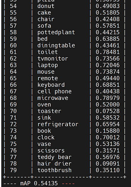
- 推論
Ubuntu では,次のコマンドを実行.
cd /usr/local/PyTorch-YOLOv3 yolo-detect --images data/samples/推論の結果が表示される. 推論の結果としては,data/samples 下にある画像ファイルについての物体検出の結果である,クラス名と確信度 (confidence) が得られる. あわせて,output の下に,物体検出の画像ファイルができる.
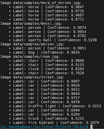
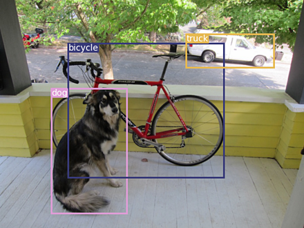
- 学習
ImageNet で事前学習済みの Darknet-53 バックエンドを用いて, COCO データセットによる学習を行う手順が, https://github.com/eriklindernoren/PyTorch-YOLOv3 で説明されている.
yolo-train --data config/coco.data --pretrained_weights weights/darknet53.conv.74
YOLOv4
物体検出のモデルである.
【関連項目】 AlexeyAB darknet, YOLOv3, YOLOX, モデル, 物体検出
Google Colaboratory で YOLOv4 による物体検出(AlexeyAB darknet を使用)
次のコマンドやプログラムは Google Colaboratory で動く(コードセルを作り,実行する)
- Google Colaboratory で,ランタイムのタイプを GPU に設定する.
- AlexeyAB darknet のビルド
%cd /content
!rm -rf darknet
!git clone https://github.com/AlexeyAB/darknet
%cd darknet
!make GPU=1 CUDNN=1 CUDNN_HALF=1 OPENCV=1
- 重みのダウンロード
AlexeyAB darknet のアセット: https://github.com/AlexeyAB/darknet/releases/
!curl -LO https://github.com/AlexeyAB/darknet/releases/download/darknet_yolo_v3_optimal/yolov4.weights - YOLOv4 による物体検出
!rm -r predictions.jpg
!./darknet detector test cfg/coco.data cfg/yolov4.cfg yolov4.weights data/dog.jpg -dont_show
from PIL import Image
Image.open('predictions.jpg').show()
!./darknet detector test cfg/coco.data cfg/yolov4.cfg yolov4.weights data/giraffe.jpg -dont_show
Image.open('predictions.jpg').show()
!./darknet detector test cfg/coco.data cfg/yolov4.cfg yolov4.weights data/horses.jpg -dont_show
Image.open('predictions.jpg').show()
!./darknet detector test cfg/coco.data cfg/yolov4.cfg yolov4.weights data/person.jpg -dont_show
Image.open('predictions.jpg').show()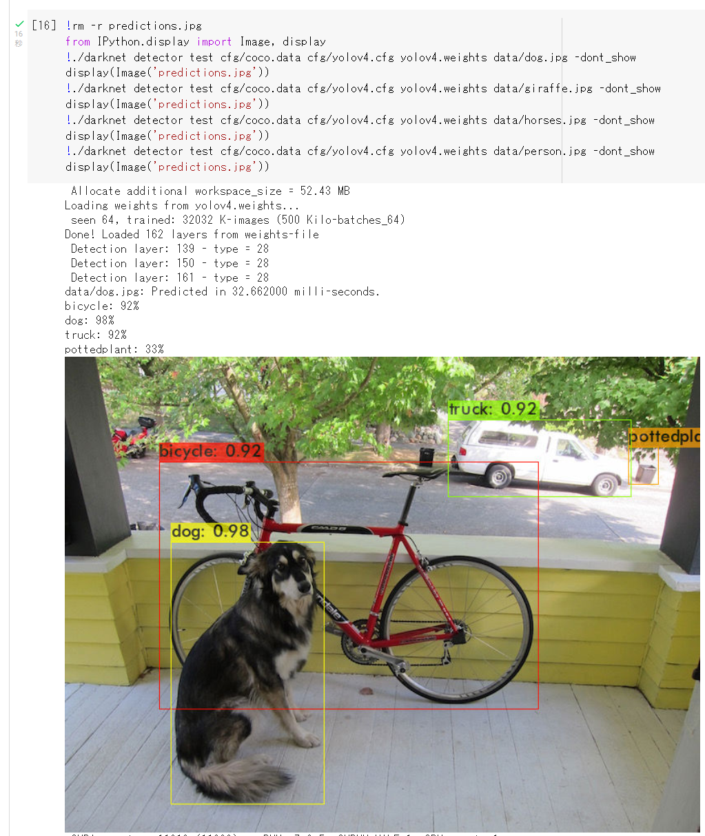
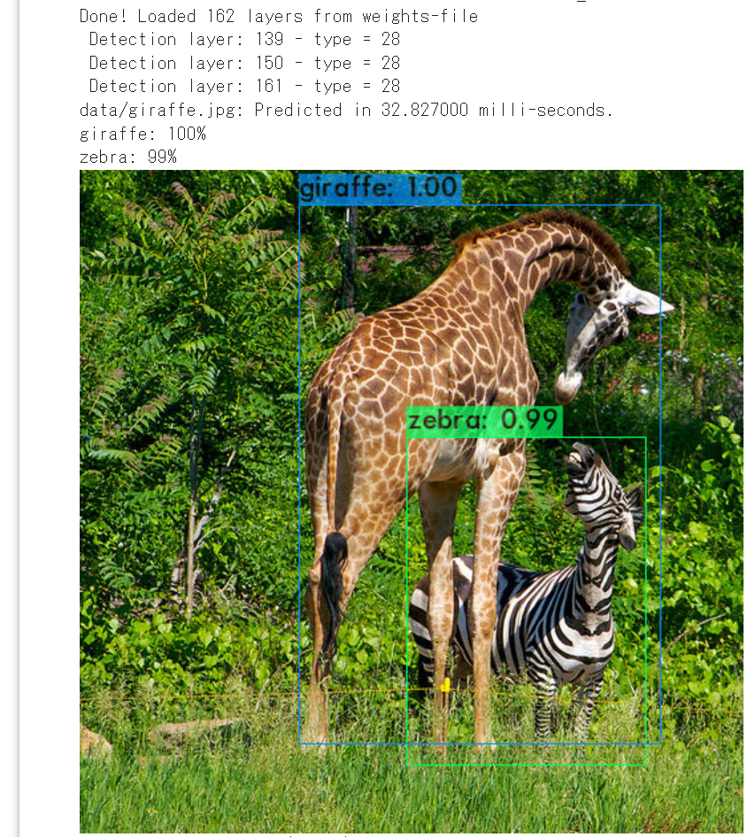
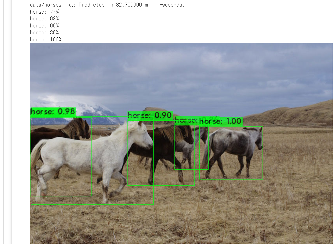
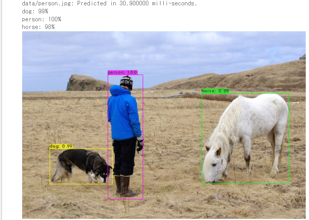
YOLOX
物体検出のモデルである. single-stage である. DarkNet53 をバックボーンとする YOLOv3 に修正を行ったものである.
- 文献
Zheng Ge, Songtao Liu, Feng Wang, Zeming Li, Jian Sun, YOLOX: Exceeding YOLO Series in 2021, CoRR, abs/2107.08430v2, 2021.
- 公式のソースコード: https://github.com/Megvii-BaseDetection/YOLOX
- Papers with Code のページ: https://paperswithcode.com/method/yolox
- MMDetection のモデル: https://github.com/open-mmlab/mmdetection/blob/master/configs/yolox/README.md
【関連項目】 MMDetection, YOLOv3, YOLOv4, モデル, 物体検出
Google Colab での YOLOX のインストールとオンライン実行
公式のソースコードを使用.
- cython, pycocotools, YOLOX のインストール
!pip3 install cython !pip3 install git+https://github.com/cocodataset/cocoapi.git#subdirectory=PythonAPI !rm -rf YOLOX !git clone https://github.com/Megvii-BaseDetection/YOLOX !pip3 install -U pip !pip3 install -r YOLOX/requirements.txt !(cd YOLOX; python3 setup.py develop) - 重みのダウンロード.
!(cd YOLOX; curl -L -O https://github.com/Megvii-BaseDetection/YOLOX/releases/download/0.1.1rc0/yolox_x.pth) - 物体検出の実行
GPU を使うときは「cpu」のところを「GPU」に変える
!(cd YOLOX; python tools/demo.py image -n yolox-x -c ./yolox_x.pth --path assets/dog.jpg --conf 0.25 --nms 0.45 --tsize 640 --save_result --device cpu)./YOLOX_outputs/yolox_x/vis_res の下に結果ができるので確認
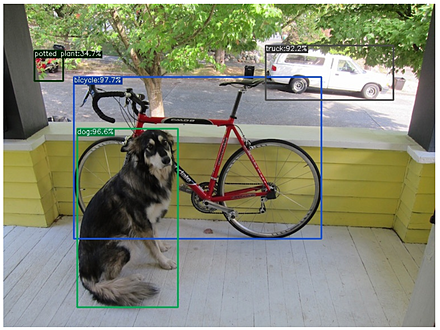
- 別の画像で物体検出の実行
GPU を使うときは「cpu」のところを「GPU」に変える
次のプログラムでは,curl は,画像ファイルのダウンロードのために用いている(コマンドを使わずに,手作業で画像ファイルを置く場合には,この部分は不要)
画像ファイル名には「../img.png」のように「../」を付けていることに注意.「../」は,「1つ上のレベルのディレクトリ」という意味.
!curl -O https://raw.githubusercontent.com/zylo117/Yet-Another-EfficientDet-PyTorch/master/test/img.png
!curl -O https://raw.githubusercontent.com/opencv/opencv/master/samples/data/fruits.jpg
!curl -O https://raw.githubusercontent.com/opencv/opencv/master/samples/data/home.jpg

!(cd YOLOX; python tools/demo.py image -n yolox-x -c ./yolox_x.pth --path ../img.png --conf 0.25 --nms \
0.45 --tsize 640 --save_result --device cpu)
!(cd YOLOX; python tools/demo.py image -n yolox-x -c ./yolox_x.pth --path ../fruits.jpg --conf 0.25 --n\
ms 0.45 --tsize 640 --save_result --device cpu)
!(cd YOLOX; python tools/demo.py image -n yolox-x -c ./yolox_x.pth --path ../home.jpg --conf 0.25 --nms\
 0.45 --tsize 640 --save_result --device cpu)
./YOLOX_outputs/yolox_x/vis_res の下に結果ができるので確認
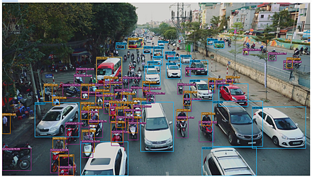
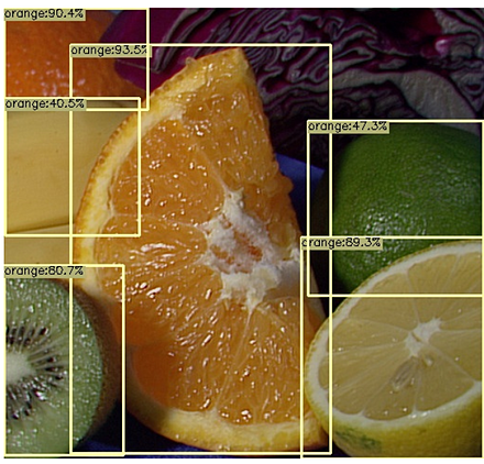
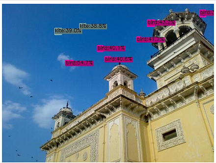
イテレーション (iteration)
モデルの学習において, モデルの重みを更新することを繰り返すが, その各々1回をイテレーション (iteration) という. 「反復」ともいう. 1回のイテレーションで,データの 1つのバッチに対する損失についてのパラメータの勾配が計算される.
インスタンス・セグメンテーション (instance segmentation)
インスタンス・セグメンテーション (instance segmentation) は, 物体検出 を行うだけでなく, 検出されたオブジェクトについて, オブジェクトのセグメンテーションマスクを画素単位で生成する.
セマンティック・セグメンテーション との違いは次の通りである. セマンティック・セグメンテーションでは,「インスタンス」という概念がないため, シーン内に複数の人物 (person) がいるような場合,人物の領域に person というラベルを付ける. インスタンス・セグメンテーションは, シーン内に複数の人物 (person) がいるような場合,それぞれの人物を分離する. 【関連項目】 セマンティック・セグメンテーション (semantic segmentation), シーン解析(scene parsing), CASILVision, MIT Scene Parsing Benchmark, 物体検出
ウエルチの方法による一元配置分散分析 (One-way analysis of means)
パラメトリック検定.等分散を仮定しない場合と仮定する場合がある.多群の検定.
なお,群数が2の場合には t 検定(R の t.test)と同じ結果が得られる.
oneway.test(x ~ y)
等分散 のときは,「var=T」を付ける.
oneway.test(x ~ y, var=T)
なお,群数が2の場合には,等分散での t 検定(R の t.test(var.equal=TRUE))と同じ結果が得られる.
【関連項目】 検定
ウィルコクソンの符号順位検定 (Wilcoxon signed-rank test)
帰無仮説: ノンパラメトリック検定の1つ.対応のある2標本で,2群の差が 0 である.
【関連項目】 検定
エポック
教師データを全て使い終わったら 1エポックである.
ミニバッチ学習を行うとき, 教師データのサイズを N とすると, N 割るバッチサイズの回数のイテレーション (iteration) が実行される. バッチサイズが 100,教師データのサイズが 800であるとすると, 8回のイテレーション (iteration) で 1エポックである.
オープンデータ (open data)
このサイトでは,「オープンデータは,インターネットで公開されているデータ,もしくは,インターネット等を用いて利用申込みができるデータ」の意味で用いている.
オープンデータには次のようなものがある.
- Aachen Day-Night データセット
- ADE20K データセット,セグメンテーション
- AFLW (Annotated Facial Landmarks in the Wild) データセット: 顔画像,21の顔ランドマーク,in-the-wild
- AIM-500 (Automatic Image Matting-500) データセット, イメージ・マッティング (image matting)
- AgeDB データセット, 顔データ,年齢, in-the-wild
- BioID 顔データベース (BioID Face Database), 顔画像,目の位置
- Caltech Pedestrian データセット,物体検出
- CelebA (Large-scale CelebFaces Attributes) データセットのダウンロード,顔検出,顔ランドマーク (facial landmark),顔認識,顔の生成
- CIFAR-10 データセット, 画像分類
- CIFAR-100 データセット, 画像分類
- Cityscapes データセット, セマンティック・セグメンテーション (semantic segmentation)
- CuRRET データベース (Columbia-Utrecht Reflectance and Texture Database), 反射率とテクスチャに関するデータベース
- COCO データセット, 物体検出 ,オブジェクトのセグメンテーション(パノプティックを含む),キーポイント,姿勢推定
- COCO の Keypoints 2014/2017 データセット, 姿勢推定
- DUTS データセット, saliency detection, salient object detection
- FaceForensics++ データセット, 画像分類
- Fashion MNIST データセット, 画像分類
- FFHQ (Flickr-Faces-HQ) データセット,顔の生成など
- FLIC (Frames Labeled In Cinema)データセット, 姿勢推定
- FordA データセット, 時系列
- FSDnoisy18k データセット, 20種類のサウンドデータ
- HELEN データセット, 顔画像,194個の顔ランドマーク
- HMDB51 (a large human motion database) データセット,行動分類,行動認識,ビデオ検索
- JHU-CROWD++ データセット, crowd counting
- ImageNet データセット, 画像分類,物体検出
- IMM 顔データベース (IMM Face Database), 顔,58個の顔ランドマーク
- iNaturalist データセット, 画像分類, 物体検出
- Iris データセット, データフレーム
- Kinetics Human Action Video データセット, ビデオでのアクション
- KITTI データセット,3次元のセグメンテーション
- ks_1033_data, データフレーム
- LFW データセット: 顔データ,人物のID,顔認識 (face recognition),in-the-wild
- LSP データセット, 姿勢推定
- LSUN (Large-scale Scene UNderstanding Challenge) データセット, 画像分類,画像生成
- Mapillary Vistas Dataset (MVD), セマンティック・セグメンテーション (semantic segmentation), インスタンス・セグメンテーション (instance segmentation)
- MIT Scene Parsing Benchmark, セマンティック・セグメンテーション (semantic segmentation), シーン解析(scene parsing),インスタンス・セグメンテーション (instance segmentation)
- LVIS データセット, シーン解析(scene parsing),インスタンス・セグメンテーション (instance segmentation)
- MNIST データセット, 画像分類
- MPII Human Pose データセット, 姿勢推定
- MUCT 顔データベース, 顔と 76 顔ランドマークのデータベース
- NWPU-Crowd データセット, crowd counting
- Objects365 データセット,物体検出
- OpenCV のサンプルデータ, 画像など
- Pascal VOC (Pascal Visual Object Classes Challenge) データセット,物体検出 ,セグメンテーション,画像分類
- PointCloudLibrary の3次元点群データ,3次元点群
- Photo Tourism データセット,Structure from Motion
- Places365 データセット,画像分類
- Reuters newswire topics データセット, ドキュメント
- SBU データセット,影検出
- ShapeNet データセット,3次元CADモデル
- ShanghaiTech データセット, crowd counting
- SVHN (The Street View House Numbers) データセット,画像分類
- Titanic データセット, データフレーム
- UCF101 (UCF101 Human Actions dataset) , ビデオでのアクション
- UCF-QNRF データセット, crowd counting
- VGGFace2 データセット,顔データ,人物のID
- WebFace260M, WebFace42M データセット,顔画像,属性付き
- WIDER FACE データセット: 顔検出
- くずし字 MNIST データセット(Kuzushiji-MNIST データセット),画像分類
- 国土数値情報,バス停留所データなど
次のデータはオープンデータではない.(ダウンロードには,申請を必要とする).
- FERET データベース, 顔画像
- Human 3.6M データセット, 姿勢推定
- iBUG 300-W データセット, 顔の 68 ランドマーク
- LS3D-W データセット, 顔ランドマーク (facial landmark)
【関連情報】
- Wikipedia の「List of datasets for machine-learning research」: https://en.wikipedia.org/wiki/List_of_datasets_for_machine-learning_research
- Papers with Code のデータセットのページ: https://paperswithcode.com/datasets
【関連項目】 R データセット (Rdatasets) を用いる場合には,
オプティカルフロー
オプティカルフローは MMFlow で算出できる.
【関連項目】 MMFlow
オプティマイザ(最適化器, optimizer)
オプティマイザは, 勾配降下法を実装したものである. 最適化器には,次のようなものがある.
- AdaGrad: ADAptive GRADient descent
- Adam: ADAptive with Momentum
TensorFlow の最適化器のベースクラスは tf.train.Optimizer クラスである.
勾配降下法の効果を高めるために,次のような手法が考案されている.
- モメンタム (momentum)
- 更新頻度 (update frequency)
- スパース性 (sparsity)
- 正則化 (Follow The (Prox-imally) Regularized Leader)
論文: An overview of gradient descent optimization algorithms, CoRR, abs/1609.04747.
http://sebastianruder.com/optimizing-gradient-descent/
Keras のオプティマイザのページ: https://keras.io/api/optimizers/
エントロピー (entropy)
print(scipy.stats.entropy([1/2, 1/2], base=2))
参考ページ: https://docs.scipy.org/doc/scipy/reference/generated/scipy.stats.entropy.html
library(entropy)
entropy(c(1/2, 1/2), unit="log2")
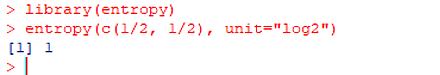
参考資料: https://cran.r-project.org/web/packages/entropy/entropy.pdf
オートエンコーダ
Undercomplete Autoencoder, Sparse Autoencoder, Convolutional Autoencoder, Stacked Autoencoder, Variational Autoencoder (VAE), VQ-VAE(Vector Quantised) などの種類がある.
キーポイント
キーポイントは,画像の中での,ある特定の特徴の座標. 「ランドマーク」ともいう.
くずし字 MNIST データセット(Kuzushiji-MNIST データセット)
くずし字 MNIST データセットは,公開されているデータセット(オープンデータ)である.
【文献】 CODH:Center for Open Data in the Humanities), KMNISTデータセット(機械学習用くずし字データセット), arXiv:1812.01718 [cs.CV], 2018.
【サイト内の関連ページ】
【関連する外部ページ】
- くずし字 MNIST データセットの公式ページ:
https://github.com/rois-codh/kmnist
Kuzushiji-MNIST, Kuzushiji-49, Kuzushiji-Kanji の 3種類が公開されている(オープンデータ).
【関連項目】 MNIST データセット, TensorFlow データセット, オープンデータ, 画像分類
Python での くずし字 MNIST データセットのロード(TensorFlow データセットを使用)
次の Python プログラムは,TensorFlow データセットから,くずし字 MNIST データセットのロードを行う. x_train, y_train が学習用のデータ.x_test, y_test が検証用のデータになる.
- x_train: サイズ 28 × 28 の 60000枚の濃淡画像
- y_train: 60000枚の濃淡画像それぞれの,種類番号(0 から 9 のどれか)
- x_test: サイズ 28 × 28 の 10000枚の濃淡画像
- y_test: 10000枚の濃淡画像それぞれの,種類番号(0 から 9 のどれか)
次のプログラムでは,くずし字 MNIST データセットのロードを行う.x_train と y_train を 25枚分表示することにより,x_train と y_train が,手書き文字のモノクロ画像であることが確認できる.
from __future__ import absolute_import, division, print_function, unicode_literals
import tensorflow as tf
import numpy as np
import tensorflow_datasets as tfds

%matplotlib inline
import matplotlib.pyplot as plt
import warnings
warnings.filterwarnings('ignore')   # Suppress Matplotlib warnings

kmnist, kmnist_metadata = tfds.load('kmnist', with_info = True, shuffle_files=True, as_supervised=True, batch_size = -1)
x_train, y_train, x_test, y_test = kmnist['train'][0], kmnist['train'][1], kmnist['test'][0], kmnist['test'][1]

plt.style.use('default')
plt.figure(figsize=(10,10))
for i in range(25):
    plt.subplot(5,5,i+1)
    plt.xticks([])
    plt.yticks([])
    plt.grid(False)
# squeeze は,サイズ1の次元を削除.numpy は tf.Tensor を numpy に変換
    plt.imshow(np.squeeze(x_train[i]), cmap=plt.cm.binary)
    plt.xlabel(y_train[i].numpy())

# 確認表示
plt.show()
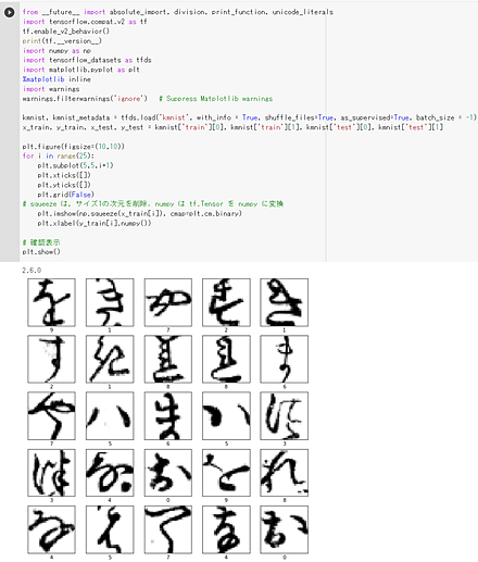
クラス
クラスはオブジェクトの種類,もしくは,同一種類のオブジェクトの集まりの意味である.
クラス番号
クラス番号は, クラスを示す番号.
クラスカル・ウォリス検定 ( Kruskal-Wallis rank sum test)
帰無仮説: ノンパラメトリック検定の1つ.対応の無い多群の差の検定
群数が2の場合には,マン・ホイットニーの U 検定と同じ結果が得られる.
kruskal.test(length ~ group)
【関連項目】 検定
コルモゴロフ–スミルノフ検定 (Kolmogorov-Smirnov test)
帰無仮説: ノンパラメトリック検定の1つ.2標本に対して使う場合には,2標本が,同一の母集団である.検定では,各標本の累積確率分布を使用.
ks.test(s1, s2)
【関連項目】 検定
コンピュータビジョンのタスク
コンピュータビジョンのタスクは種々があるが,次のようなものをあげることができる.
- シーン
- シーン理解 (scene parsing)
- 画像分類 (image classification)
- image tagging (weather tagging, scene tagging などがある)
- Class Activation Mapping (CAM)
- セマンティック・セグメンテーション (semantic segmentation), pixelwise classification ともいう
- インスタンス・セグメンテーション (instance segmentation)
- パノプティックセグメンテーション (panoptic segmentation)
- 物体検出 (object detection)
- salient object detection
- シーン解析(scene parsing)
- Few Shot Segmentation
- 動画像の処理
- multi object tracking
- segmentation tracking
- optical flow
- 画像や動画の編集
- image inpainting
- 画像のノイズ除去 (image restoration)
- イメージ・マッティング (image matting)
- 超解像 (super resolution)
- generation
- image content removal(画像コンテンツの除去)
- 人物検出,姿勢推定
- 人物検出(human detection)
- 姿勢推定(pose estimation)
- 頭部姿勢推定(head pose estimation)
- 顔情報処理
- 動作認識
- スケルトンベースの動作認識 (skelton-based action recognition)
- Spatio-Temporal Action Recognition
- ビデオの動作認識 (action recognition)
- 3次元再構成
- テキスト
- テキスト検知 (text detection)
- テキスト認識 (text recognition)
シーン解析(scene parsing)
シーン解析(scene parsing) では,画像全体の画素をクラスに分類する.各画素にクラスのラベルが割り当てられる. セマンティック・セグメンテーション (semantic segmentation) との違いとしては,画像全体の画素を何らかのクラスに分類する(クラスが不明な画素が無い)ことである.
【関連項目】 セマンティック・セグメンテーション (semantic segmentation)
シグモイド関数 (sigmoid function)
シグモイド関数 (sigmoid function) は,次の関数である.
f(x) = 1 / (1 + exp(-x))
シグモイド関数は,活性化関数としてよく使用されるもののうちの1つである. 活性化関数は,ニューロンの入力の合計から,そのニューロンの活性度の値を決めるためのもの. (他には,ReLU,LReLU,ステップ関数,ソフトマックス関数などがある.)
シャピロ・ウィルク検定 (Shapiro Wilk test)
帰無仮説: 標本の母集団は正規分布である
s1 <- iris[iris$Species=='setosa',]$Sepal.Length
s2 <- iris[iris$Species=='versicolor',]$Sepal.Length
s3 <- iris[iris$Species=='virginica',]$Sepal.Length

shapiro.test( s1 )
shapiro.test( s2 )
shapiro.test( s3 )
【関連項目】 検定
ステップ関数 (step function)
ステップ関数は,次の関数である.
f(x) = 0 (x < 0 のとき), 1 (x >= 0 のとき)
セマンティック・セグメンテーション (semantic segmentation)
セマンティック・セグメンテーション (semantic segmentation)では, 画像内に人物 (person) がいるような場合,人物の領域に person というラベルを付ける. このとき,人物は複数いても問題ない.
学習のときには,'road', 'slidewalk', 'building' のようなクラスについての学習を行う. 学習データでは,画像の画素に,'road', 'slidewalk', 'building' のようなクラス名(あるいはクラス番号)がラベルとして付いている. 学習済みデータで推論を行うと,画素に 'road', 'slidewalk', 'building' のようなラベルが付く.
road, sidewalk, parking, rail track, person, rider, car, truck, bus, on rails, motorcycle, bicycle, caravan, trailer, building, wall, fence, guard rail, bridge, tunnel, pole, pole group, traffic sign, traffic light, vegetation, terrain, sky, ground, dynamic, static
【関連項目】 ADE20K データセット, BASNet (Boundary-Aware Salient object detection), BDD100K, CSAILVision, Cityscapes データセット, COCO (Common Object in Context) データセット, DeepLab2, DeepLabv3, DeepLabv3+, Mapillary Vistas Dataset (MVD), MIT Scene Parsing Benchmark, MMSegmentation, OCRNet, Pascal VOC (Pascal Visual Object Classes Challenge) データセット, Residual Networks (ResNets), SegFormer, U-Net, インスタンス・セグメンテーション (instance segmentation), コンピュータビジョンのタスク, シーン解析(scene parsing), 物体検出
ソフトマックス関数 (softmax function)
次元数 n のベクトル x に対するソフトマックス関数 (softmax function) は,f(x[k]) = exp(x[k]) / (exp(x[1]) + exp(x[2]) + ... exp(x[n]))
ニューラルネットワークの,ある層(レイヤ)の出力が one-hot 表現の出力であるときによく使用される.
チェックポイント
ある特定の時点での,モデルの変数の状態を表したデータのこと. チェックポイントにより,ニューラルネットワークの重み (weight) をエクスポートすることができるようになる.
データサイエンス
データサイエンスというとき,データを数理的に処理(事前に定義された数式に当てはめて処理)することにより, 処理された結果が,どのようにして算出されたかが明らかであり,算出に再現性があるという意味合いに加えて, その数理的処理において,体系だった学問があるという意味がある.
データサイエンスでは,次のようなものを扱う.
記述統計量,分布,相関,正規化,外れ値,クラスタリング,統計処理
データの前処理
TensorFlowでは,入力の値が 0 から 1 の範囲の浮動小数点数にスケールする必要がある.
データフレーム
データフレームでは,データのデータ型は,列ごとに同じである. 列に属性名がある.
【関連項目】 Iris データセット, ks_1033_data, titanic データセット, ポケモンデータセット
データ拡張 (data augmentation)
データ拡張 (data augmentation)では,すでに存在するデータを利用して,データを変換することにより,データを増量する.
ディープラーニング
ディープラーニングは,層の浅いニューラルネットワークの組み合わせによる多層性の実現により勃興した分野. ジェフ・ヒントンらが見出したオートエンコーダやディープ・ビリーフ・ネットワークが基礎である.
【関連項目】 applications of deep neural networks, cnn (convolutional neural network), gan (generative adversarial network), gru (gated recurrent neural networks), keras, lstm (long short-term memory), pytorch, tensorflow, ニューラルネットワーク, 強化学習, 層構造のニューラルワーク
ディープニューラルネットワーク
ディープラーニングを行う ニューラルネットワーク. 「ディープモデル (deep model)」ともいう.
ドロップアウト
学習の途中で, ニューラルネットワークを構成するニューロンを無作為(ランダム)に「あたかも存在しない状態」にすること. 過学習の防止に効果がある場合があるとされる.
参考文献: dropout: a simple way to prevent neural networks from overfitting, https://www.cs.toronto.edu/~rsalakhu/papers/srivastava14a.pdf
参考文献: improving neural networks by preventing co-adaptation of feature detectors, corr, abs/1207.0580
ニューラルネットワーク
ニューラルネットワークは,人間の脳細胞を,信号が流れるネットワークと見立てたうえで, 個々の脳細胞を, 次の簡単な数理で組み立てるもの.
ニューラルネットワークは,入力を与えると, 出力が出てくる. この仕組みにより,質問が与えられたときに,多数の選択肢の中から 1つを選ぶことなどもできる. 例えば,コンピュータに画像を見せて「男か女か」の答えを出す,年齢を「0から120の中から」答えるということができる.
ニューラルネットワークは層で構成されている.隠れ層を持つのがふつうである. ニューロンには非線形性がある.
ニューラルネットワークでは, 前もって,入力とそれに対する正解についての学習を行うことによって, 入力に対して,適切な出力が出てくるにようになる.
ニューラルネットワークは 1980年代に登場した. ニューラルネットワークの技術革新としては,次のようなものがある.
- ドロップアウトや正規化などによる過学習の防止
- relu法により,ニューラルネットワークの本質的課題であった勾配消失問題の解決
- gpuプロセッサの活用
- early stoppingなどの正則化のための手法
以上の背景から,ディープニューラルネットワークが広く使われるようになった.
【関連項目】 applications of deep neural networks, ディープラーニング
ニューラルネットワークのビジュアライズ
keras visualizer を用いて keras のニューラルネットワークをビジュアライズするプログラムは次の通り.
from keras_visualizer import visualizer
visualizer(m, format='png')
from PIL import Image
Image.open('graph.png').show()
windows の場合は,コマンドプロンプトを管理者として開き次のコマンドを実行する.
python -m pip install git+https://github.com/lordmahyar/keras-visualizer
google colaboratory では「!pip3 install git+https://github.com/lordmahyar/keras-visualizer」を実行
!pip3 install git+https://github.com/lordmahyar/keras-visualizer
ニューラルネットワークの種類
ニューラルネットワークの種類には,次のようなものがある. 「教師あり」は,教師データを用いての 学習の機能があるもの. 「教師なし」は,そうでないものである.
- 教師あり
- 教師なし
オートエンコーダ (autoencoder)
ニューラルネットワークのビジュアライズ
keras のモデルのビジュアライズについては: https://keras.io/ja/visualization/
import pydot
plot_model(m)
ニューロン (neuron)
ニューロンは, 複数の入力の総和に,バイアス (bias)を足したのち,ニューロンに設定された活性化関数を適用して得られた値を出力する. ニューロンの入力と出力の間には 重みがある. ニューロンの出力には,重みが掛け合わされたのちに,次のニューロンの入力になる.
1つのニューロンは,複数の入力を取ることができる.出力は1つである.これら入力と出力は,次のいずれかの条件を満たす
- ある特定のニューロンを見ると,すべての入力は,1つの数である.出力も1つの数である.
- ある特定のニューロンを見ると,すべての入力は,数のベクトルである.出力も数のベクトルである.そして,それらの次元数がすべて等しい.
層構造のニューラルワークでは, バイアスは,ニューロンごとに違い, 活性化関数は,同じ層(レイヤ)のニューロンでは同じものとするのが通例.
ニューロンの発火
ニューロンの発火は, 1 あるいは 1 に近い高い値を出力すること.
パーセプトロン (perceptron)
パーセプトロンは,1つまたは複数の入力を取り,入力値の加重和に対して関数を実行し,1つの出力値を計算するシステムである. 機械学習では,関数として,relu,シグモイド関数などの非線形関数を用いることが多い. 例えば,以下のパーセプトロンでは,x1, x2, x3, x4, x5 の加重和に対してシグモイド関数を実行し,出力値を得るものである. f(x1, x2, x3, x4, x5) = sigmoid(w1x1 + w2x2 + w3x3 + w4x4+ w5x5)
ニューラルネットワークは, 複数のパーセプトロンを接続したネットワークであり, バックプロパゲーションによりフィードバックを行う.
バイアス (bias)
次の式では,b はバイアスである.
y = b + w1 * x1 + w2 * x2 + ... + wn * xn
ニューラルネットワークでのバイアスは個々のニューロンが持つ値.ニューロンの発火のしやすさを表す値とされる.
ハイパーパラメータ (hyper parameter)
ハイパーパラメータは,次の 2つである.
- モデルパラメータ
層(レイヤ)の数,各層のニューロンの数など
- アルゴリズムパラメータ
学習アルゴリズムに関するパラメータ
ハイパーパラメータチューニング
最適なハイパーパラメータを探索すること.
ハイパーパラメータチューニングを行うモデルの定義
ハイパーパラメータチューニングを行うモデルの定義では, ハイパーパラメータの探索を行う探索空間を定義する.
iris データセット を,3種類に分類する keras プログラムの例は次の通り.
from __future__ import absolute_import, division, print_function, unicode_literals
import tensorflow as tf
from tensorflow.keras import layers
import numpy as np
from sklearn.datasets import load_iris
import sklearn.model_selection
from sklearn.preprocessing import normalize
from IPython.display import display

gpu = tf.config.list_physical_devices(device_type = 'GPU')
if len(gpu) > 0:
    print("GPU:", gpu[0].name)
    tf.config.experimental.set_memory_growth(gpu[0], True)

# データ
num_classes = 3

iris = load_iris()
x = iris.data
y = iris.target

x_train, x_test, y_train, y_test = sklearn.model_selection.train_test_split(x.reshape(x.shape[0], -1), y, train_size=0.5)

m = tf.keras.Sequential(
    [
        layers.Dense(units=64, input_dim=len(x_train[0]), activation='relu'),
        layers.Dropout(0.5),
        layers.Dense(num_classes, activation="softmax"),
    ]
)

print(m.summary())

batch_size = 4
epochs = 300

m.compile(
    optimizer=tf.keras.optimizers.Adam(learning_rate=0.001),
    loss='sparse_categorical_crossentropy',
    metrics=['sparse_categorical_crossentropy', 'accuracy']
)

history = m.fit(x_train, y_train, batch_size=batch_size, epochs=epochs, validation_data=(x_test, y_test))

score = m.evaluate(x_test, y_test, verbose=0)
print("Test loss:", score[0])
print("Test accuracy:", score[1])

# 分類
predictions = m.predict(x_test)
print(predictions.argmax(axis=1))
# 正解の表示
print(y_test)

import pandas as pd
h = pd.DataFrame(history.history)
h['epoch'] = history.epoch
print(h)

# 学習曲線
# https://www.tensorflow.org/tutorials/keras/overfit_and_underfit?hl=ja で公開されているプログラムを使用
%matplotlib inline
import matplotlib.pyplot as plt
import warnings
warnings.filterwarnings('ignore')   # Suppress Matplotlib warnings

def plot_history(histories, key='binary_crossentropy'):
  plt.figure(figsize=(16,10))

  for name, history in histories:
    val = plt.plot(history.epoch, history.history['val_'+key],
                   '--', label=name.title()+' Val')
    plt.plot(history.epoch, history.history[key], color=val[0].get_color(),
             label=name.title()+' Train')

  plt.xlabel('Epochs')
  plt.ylabel(key.replace('_',' ').title())
  plt.legend()

  plt.xlim([0,max(history.epoch)])

plot_history([('history', history)], key='sparse_categorical_crossentropy')
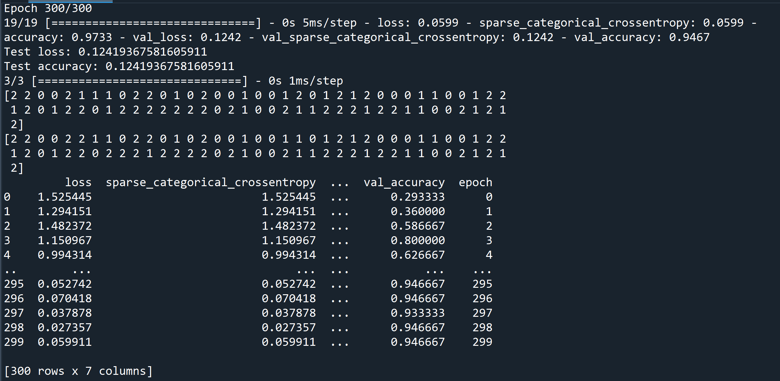
バウンディングボックス (bounding box)
写真やビデオの中での,対象領域を示す矩形. 取り扱いたい対象を囲むような矩形を作ることが多いことから「バウンディング」と呼ばれる.
バッチ (batch)
バッチ (batch) は, ミニバッチ学習 での 学習の1回のイテレーション (iteration) で使われるデータ集合などのこと.
バックプロパゲーション (backpropagation)
バックプロパゲーション (backpropagation) は, ニューラルネットワークで,勾配降下法 (gradient descent) を実行するためのアルゴリズムである. パラメータと損失の偏微分を算出することにより,バックプロパゲーションが実行される.
バッチサイズ (batch size)
1つのバッチ (batch) の中のデータ等の数のこと. 確率的勾配降下法 (sgd 法) のバッチサイズは 1 である. ミニバッチ学習 でのバッチサイズは普通 10 から 100 である.
バッチ正規化 (batch normalization)
バッチ正規化 (batch normalization) は, ミニバッチ学習を行うとき,ミニバッチごとに, 隠れ層 (hidden layer) の活性化関数の入力や出力を, 正規化すること. 過学習 (overfitting) の緩和などの効果がある.
バッチ正規化 (batch normalization) の代替とされる手法(adaptive gradient clipping 法など)も登場しつつある.
【keras のプログラム】
from __future__ import absolute_import, division, print_function, unicode_literals
import tensorflow as tf
m = tf.keras.sequential()
m.add(tf.keras.layers.flatten(input_shape=(28, 28)))
m.add(tf.keras.layers.dense(units=128, activation='relu'))
m.add(tf.keras.layers.batchnormalization())
m.add(tf.keras.layers.dropout(0.5))
m.add(tf.keras.layers.dense(units=10, activation='softmax'))
ソフトマックス関数 (softmax function)を活性化関数とするような層(レイヤ)では,batchnormalization は行わないようです.
- batch normalization: accelerating deep network training by reducing internal covariate shift, corr, abs/1502.03167
パラメータ (parameter)
機械学習でのパラメータは, モデルの変数のうち,機械学習のシステムでの学習の対象になっているもの. モデルの変数でも,学習の対象になっていないものはハイパーパラメータである.
プーリング (pooling)
直前の畳み込み層で生成された1つの行列(あるいは複数の行列)を,より小さな行列に縮小すること
フィードフォワード (feed forward)
ある層のニューロンでの結果を,次の層のニューロンが受け取る (それ以外にはない)ような構造になっているような ニューラルネットワークを「フィードフォワード」という.
ポケモンデータセット
ポケモンデータセットの url: https://gist.github.com/armgilles
次の Python プログラムは,ポケモンデータセットの主成分分析を行い,第1主成分,第2主成分,第3主成分,ポケモンデータセットの属性 Type 1 で3次元の散布図を表示する.
次の Python プログラムでは,3次元の散布図のために, plotly の scatter_3d を用いている.
!git clone https://gist.github.com/armgilles/194bcff35001e7eb53a2a8b441e8b2c6
!mv 194bcff35001e7eb53a2a8b441e8b2c6/pokemon.csv .

import numpy as np
import pandas as pd
from sklearn.datasets import load_iris
import sklearn.decomposition
%matplotlib inline
import matplotlib.pyplot as plt
import warnings
warnings.filterwarnings('ignore')   # Suppress Matplotlib warnings
import plotly.express as px
from IPython.display import display

pokemon = pd.read_csv("pokemon.csv")
display(pokemon)

x = pokemon.iloc[:,4:11].to_numpy()
type1 = pokemon.iloc[:,2]
pca = sklearn.decomposition.PCA(n_components=4)
r = pca.fit_transform(x)

fig = px.scatter_3d(x=r[:,0], y=r[:,1], z=r[:,2], color=type1, symbol=type1, opacity=0.4,
                 labels={'x': '1', 'y': '2', 'z': '3', 'color': 'Type 1', 'symbol': 'Type 1'})
fig.show()
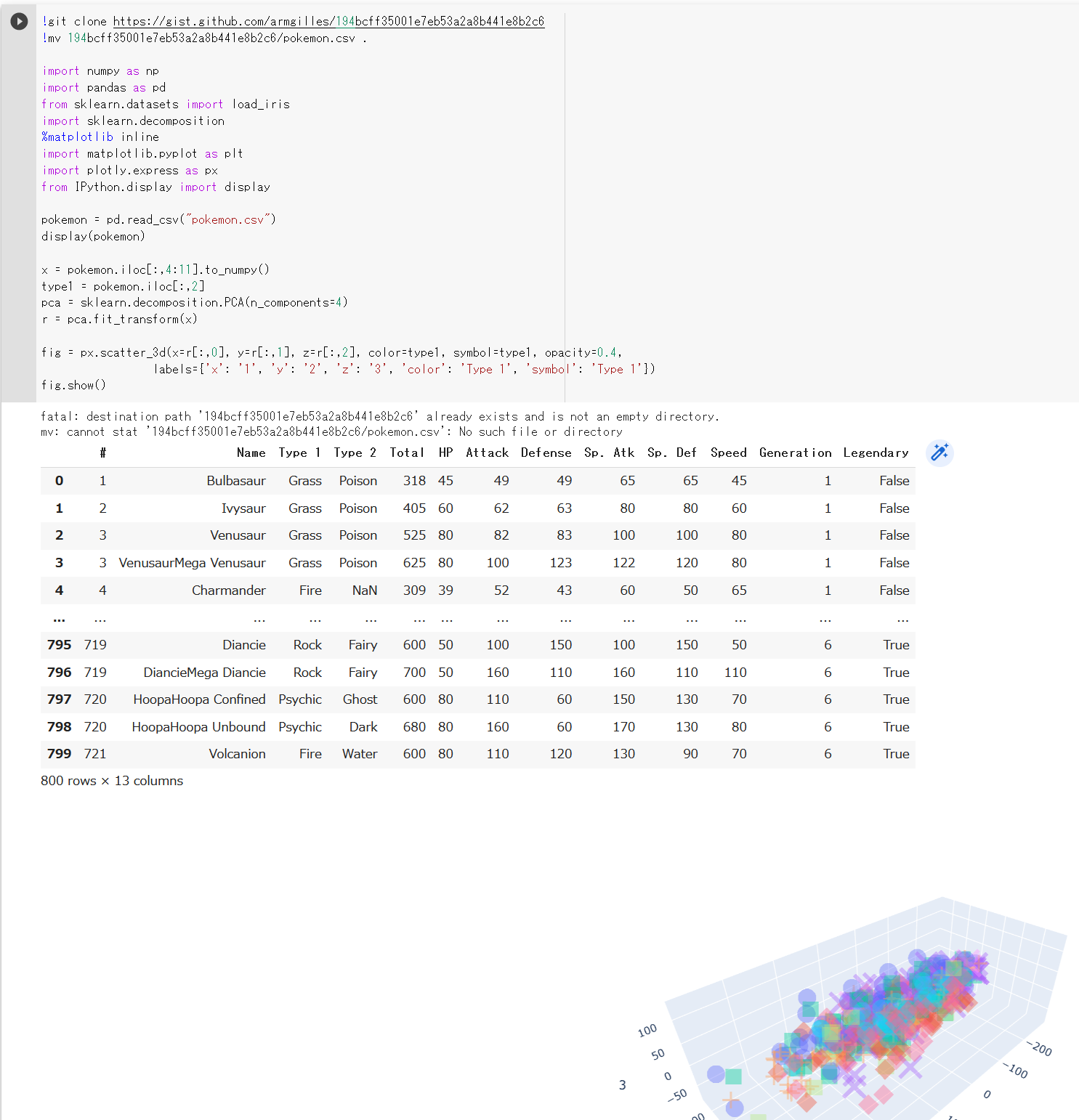
マスク付き顔の処理
マスク付き顔の処理には次のようなものがある.
- マスク付き顔の顔検知
- マスク付き顔の顔検知,マスクなし顔の顔検知を同時に行うもの: Chandrika Deb の顔マスク検出 (Chandrika Deb's Face Mask Detection)
【関連項目】 cabani の MaskedFace-Net データセット, Chandrika Deb の顔マスク検出 (Chandrika Deb's Face Mask Detection)
マスターフェイス (master face)
マスターフェイス (master face)は,顔認識 (face recognition)のシステムにおいて, そこに登録された顔のテンプレートの複数にマッチ (match) するような顔.
顔認識のシステムは,他人の顔を間違って認識したり,あるいは人工知能が合成した顔を間違って認識したりすることがありえるものである.
近年,種々の研究があり, 「Dlib, FaceNet, SphereFace の 3つの顔認識システムについて, 10未満のマスターフェイスが,LFW データセットの 40 パーセント以上にマッチする」という報告もある. (コメント:Dlib, FaceNet, SphereFace の優劣や評価ではなく,現行の顔認識システム全般の脆弱性の指摘であると受け止めることができると,本サイト作成者は考えています).
- 文献
Huy H. Nguyen, Sébastien Marcel, Junichi Yamagishi, Isao Echizen, Master Face Attacks on Face Recognition Systems, CoRR, abs/2109.03398v1, 2021.
- 文献
Ron Shmelkin, Tomer Friedlander, Lior Wolf, Generating Master Faces for Dictionary Attacks with a Network-Assisted Latent Space Evolution, CoRR, abs/2108.01077v3, 2021.
【関連項目】 顔識別 (face identification), 顔認識 (face recognition), 顔に関する処理
マン・ホイットニーの U 検定 (Mann-Whitney U test, Wilcoxon rank sum test)
帰無仮説: ノンパラメトリック検定の1つ.独立な2標本で,2標本が同じ母集団から得られた標本である.
wilcox.test(s1, s2)
なお,correct=F を付けると,連続性の修正(continuity correction)を行わないようになる.
wilcox.test(s1, s2, correct=F)
【関連項目】 検定
ミニバッチ (mini-batch)
学習の繰り返しのうち,各々の繰り返しで使用されるバッチ全体の中からランダムに選ばれた部分集合である. ミニバッチのバッチサイズは,ふつう,10 から 1000 である. ミニバッチの使用により,損失の計算を高速化できるとされている.
ミニバッチ学習
ミニバッチ学習は,教師データの中から,「バッチ」あるいは「ミニバッチ」と呼ばれる少数を無作為に(ランダムに)選び出し,それを使って学習を行うこと.
ミニバッチ確率勾配降下法 (mini-batch stochastic gradient descent)
ミニバッチを使用する確率勾配降下法である. 学習データのミニバッチを用いて,勾配が算出される. 通常の確率的勾配降下法は,サイズ1のミニバッチを使用するミニバッチ確率勾配降下法と同じである.
メトリクス(metrics)
メトリクスは,モデルの性能を判定するための関数である. メトリクスは,損失関数とは違い,学習時には使用されない.
Keras では,メトリクスは,関数のリストである.そして,Keras では,任意の損失関数をメトリクスとして使うことができる.
Keras のメトリクスのページ: https://keras.io/api/losses/index.html
モデル
機械学習での「モデル」は, 機械学習のシステムが教師データを用いて学習した内容を表現したものである.
TensorFlowでは,「モデル」は次のような意味でつかわれる場合がある. ・TensorFlow グラフは,ニューラルネットワークによる予測がどのように計算されるかの構造を表現したもの. ・TensorFlow グラフの重みとバイアスの値は,学習により決定される.
ディープニューラルネットワークのモデルには,次のようなものがある.
- DeepLab2
- DeepLabv3
- DenseNet121, DenseNet169: 画像分類
- Hour Glass Network
- Inception-v4: 画像分類
- Inception-ResNet: 画像分類
- MixConv
- MobileNetV2: 画像分類
- MobileNetV3: 画像分類
- NASNet: 画像分類
- ResNet50, ResNet101, ResNet152, その他の ResNet: 画像分類
- ResNeXt: 画像分類
- RetinaNet
- SpineNet
- TinaFace
- Wide ResNet: 画像分類
- Xception
- YOLOv3: 物体検出
【関連項目】 PyTorch, torchvision のモデル, rwightman の PyTorch Image Models (TIMM)
モメンタム (momentum)
ある学習ステップは,現在のステップでの勾配だけでなく, その直前のステップの勾配にも依存するという考え方による勾配降下法. モメンタムでは,時間経過に伴いながら,勾配の指数加重移動平均を算出する.
ラベル (label)
ラベルは,クラスの番号やクラス名など,クラスを識別できる番号や文字列などのこと.
ロジット
分類の結果として得られる数値ベクトルで,正規化されていないもの. ロジットに対しては,正規化が行われるのが普通である.
多クラスの分類では,ロジットを正規化するために ソフトマックス関数 (softmax function)を用いるのが普通である. ソフトマックス関数 (softmax function)により,数値ベクトルが生成されるが,そのそれぞれの値が1クラスに対応する.
ロジットの別の意味として,ロジットという言葉を,ロジット関数(シグモイド関数 (sigmoid function))という意味で使うことがある.
重み (weight)
線形モデルでの特徴での係数である. ニューラルネットワークで,あるニューロンとニューロンが結合しているとき, 個々の結合には重みがある. 重みが大きいほど,当ニューロンの出力が強く,次のニューロンに渡される. 例えば, あるニューロンが,別の2つのニューロンと結合していて,それら2つの出力を受け取るとき, そのニューロンの入力は,w[1] * x[1] + w[2] * x[2] のようになる. w[1], w[2] は重み, x[1], x[2] は2つのニューロンの出力である.
重みの初期化
重みの初期化 (weights initialization)
重みの方向ベクトル
重みが複数あるとき,それらは重みの方向ベクトルをなす. 重みが複数あり,それら重みをそれぞれ増やしたり減らしたりする量は,重みの方向ベクトルをなす.
音声処理のタスク
音声処理のタスクには次のようなものがある.
- audio source separation
- music source separation
- speech enhancement
- Speech synthesis
- 音声合成 (Text To Speech; TTS)
音声合成 (Text To Speech; TTS)
人間の音声を合成すること.
【関連項目】 Coqui TTS, Speech synthesis, VALL-E X, VOICEVOX, 自然言語処理のタスク
解釈可能性 (interpretability)
モデルを用いた予測について,それが容易に説明できるかの度合い.
顔に関する処理
顔に関する処理には,次のようなものがある.
- 3次元の顔の再構成 (3D face reconstruction)
- 顔検証 (face verification)
- 顔検出 (face detection)
- 顔識別 (face identification)
- 顔認識 (face recognition)
- 顔の 68 ランドマーク の検出
- 顔のコード化
- 顔の性別,年齢等の予測
- 顔ランドマーク (facial landmark)の検出
- 顔ランドマークの3次元化
顔のコード化
顔のコード化では,顔を数値(複数の数値)に置き換える. このとき,同一人物の顔は,近い値の数値に, 違う人物の顔は,離れた値の数値になるようにコード化を行う.
顔のデータベース
顔のデータベースの有名なものには,
- AgeDB データセット, 顔データ,年齢, in-the-wild
- AFLW (Annotated Facial Landmarks in the Wild) データセット: 顔画像,21の顔ランドマーク,in-the-wild
- CelebA (Large-scale CelebFaces Attributes) データセットのダウンロード
- FFHQ (Flickr-Faces-HQ) データセット(顔認識)
- LFW データセット: 顔データ,人物のID,顔認識 (face recognition),in-the-wild
- LSUN (Large-scale Scene UNderstanding Challenge) データセット
- UTKFace データセット
- WebFace260M, WebFace42M データセット,in-the-wild を含む
- WIDER FACE データセット: 顔検出
などがある.これらの中には,シナリオが「in-the-wild」であるもの,顔が部分しか見えていないものを含むようなデータセットもある.
その他,マスク付きの顔のデータセットには, cabani の MaskedFace-Net データセット, Chandrika Deb の顔マスク検出 (Chandrika Deb's Face Mask Detection) および顔のデータセット などがある.
その他,顔のデータセットは, 300W (300 Faces-In-The_Wild) データセット, AgeDB データセット, C-MS-Celeb Cleaned データセット , FERET データベース, HELEN データセット, iBUG 300-W データセット, IMM 顔データベース (IMM Face Database), MS-Celeb-1M データセット, MUCT 顔データベース, VGGFace2 データセットなどがある.
【関連項目】 オープンデータ
顔の性別,年齢等の予測
画像から顔の性別,年齢等の予測を行う.
顔検出 (face detection)
顔検出 (face detection)は,写真やビデオの中の顔を検出すること.顔とそれ以外のオブジェクトを区別することも行う.
顔検出 (face detection)の結果は, バウンディングボックスで得られるのが普通である.
【関連項目】 Chandrika Deb の顔マスク検出, Dlib の顔検出, Emotion-Investigator, InsightFace, RetinaFace, SCRFD (Sample and Computation Redistribution for Face Detection), TinaFace, WIDER FACE データセット, 顔検証 (face verification), 顔識別 (face identification), 顔認識 (face recognition), 顔に関する処理, 物体検出
顔検証 (face verification)
顔検証 (face verification)は, 顔と顔とを比べてマッチするか(同一人物であるか)を調べること. 本人確認などで 顔検証 (face verification) が行われる.
【関連項目】 ArcFace 法, MobileFaceNets, マスターフェイス (master face), 顔検出 (face detection), 顔識別 (face identification), 顔認識 (face recognition), 顔に関する処理
顔識別 (face identification)
顔識別 (face identification)では,ある顔と,データベースの中の多数の顔についての情報を用いて, 顔が誰であるのかの個人の特定を行う. このとき,データベースの中の多数の顔とのマッチングが行われる.
【関連項目】 ArcFace 法, マスターフェイス (master face), 顔検証 (face verification), 顔検出 (face detection), 顔認識 (face recognition), 顔に関する処理
顔認識 (face recognition)
顔認識 (face recognition)は, 写真やビデオについて顔検出 (face detection)を行い, その結果として得られた顔について(複数の顔が得られた場合にはそれぞれについて), 顔識別 (face identification) を(データベースの中の多数の顔についての情報を用いての,個人の特定)を行う.
【関連項目】 ArcFace 法, LFW データセット, マスターフェイス (master face), 顔検証 (face verification), 顔検出 (face detection), 顔識別 (face identification), 顔に関する処理
顔ランドマーク (facial landmark)
顔ランドマーク (facial landmark)は, 顔について,目,眉,鼻,口,あごのラインなどのアノテーションを行ったもの. 目,眉,鼻,口,あごのラインなど,顔のパーツの構造を特定できる形状予測器 (shape predictor) の学習に使うことができる.
【関連項目】 AFLW (Annotated Facial Landmarks in the Wild) データセット, UTKFace データセット, 顔に関する処理, 顔の 68 ランドマーク, 顔ランドマークの3次元化
顔ランドマークの3次元化
ディープラーニングを用いて 顔ランドマーク (facial landmark)の3次元化する学習済みモデルは,次のページで公開されている.
https://www.adrianbulat.com/face-alignment
【関連項目】 顔ランドマーク(facial landmark)
過学習 (overfitting)
教師データにはよく適合しているが,新しいデータに対しては,正しい予測ができないようなモデルを生成すること.
過学習では, 訓練データでは精度が高く,損失が少ないが, 検証データでは精度が低く,損失が多いというように,訓練データと検証データでの乖離が起きている.
学習 (learning)
学習は,より正しい出力が得られるように, ニューラルネットワークの重みとバイアスを修正すること. あるいは, 最適な出力が得られるように, 重みとバイアスを最適化すること.
そのために,教師データのうち,入力を使い, ニューラルネットワークを動かす. そして,正解の出力を使い, 損失関数の値ができるだけ小さくなるように, オプティマイザ(最適化器)を用いて, ニューラルネットワークを構成するニューロンの重みとバイアスなど, ニューラルネットワークのパラメータを修正する.
学習曲線 (learning curve)
学習済みモデル (trained model)
学習不足 (underfitting)
学習不足の原因は種々あり得る.
学習率 (learning rate)
勾配降下法を用いてモデルの学習を行うときに使用される値である. 勾配降下法では,イテレーションごとに,勾配と学習率の掛け算を行う. その結果として得られる積を「gradient step」と言う. 学習率は,ハイパーパラメータの1つである.
学習率をダイナミックに変化させる技術には, AdaDelta 法,Adam 法などが知られる.
確率勾配降下法 (SGD, stochastic gradient descent)
バッチサイズが 1として,勾配降下法を実行すること. これは,教師データから,ランダムに1つを選び,勾配を算出して,学習を行う.
確率的勾配降下法 (SGD 法) は,次の方法で行う勾配降下法である.
- ミニバッチ学習を行う.
- 次の手順により,損失関数の値ができるだけ小さくなるように,ニューラルネットワークの重みの値を定める
m.compile(
    optimizer=tf.keras.optimizers.SGD(learning_rate=0.0001, momentum=0.9, nesterov=True),
    loss='sparse_categorical_crossentropy',
    metrics=['sparse_categorical_crossentropy', 'accuracy']
)
隠れ層 (hidden layer)
ニューラルネットワークで,入力層と出力層の間の層.
画素
MNIST データセットは,濃淡画像 70000枚である.その画素は 0 から 255 の値になっている.
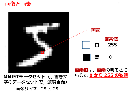
画像全体は配列として扱うことが多い.
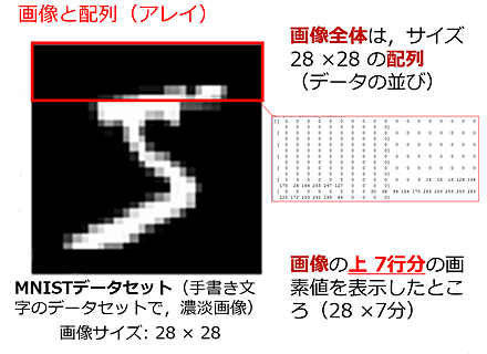
画像データのデータ拡張 (image data augmentation)
CIFAR-10 データセットについて,データ拡張のために フリップと回転を行う Keras のプログラムは次の通りである.
from __future__ import absolute_import, division, print_function, unicode_literals
import tensorflow as tf
import numpy as np
import tensorflow_datasets as tfds

# CIFAR-10 データセットのロード
cifar10, cifar10_metadata = tfds.load('cifar10', with_info = True, shuffle_files=True, as_supervised=True, batch_size = -1)
x_train, y_train, x_test, y_test = cifar10['train'][0], cifar10['train'][1], cifar10['test'][0], cifar10['test'][1]
print(cifar10_metadata)

# 増量
INPUT_SHAPE = [32, 32, 3]
data_augmentation = tf.keras.Sequential()
data_augmentation.add(tf.keras.layers.experimental.preprocessing.RandomFlip("horizontal", input_shape=INPUT_SHAPE))
data_augmentation.add(tf.keras.layers.experimental.preprocessing.RandomRotation(0.1))

def f(x):
    tf.reshape(data_augmentation(tf.reshape(x, (1, INPUT_SHAPE[0], INPUT_SHAPE[1], INPUT_SHAPE[2]))), (INPUT_SHAPE[0], INPUT_SHAPE[1], INPUT_SHAPE[2]))

display([*map(f, x_train)])
画像分類 (image classification)
画像分類は,画像からそのクラス名を求めるもの.
Big Transfer ResNetV2, CSPNet, MobileNetV2, MobileNetV3, Inception-ResNet, ResNet50,ResNet101,ResNet152, ResNeXt, DenseNet121,DenseNet169, NASNet, Vision Transformer, Wide ResNet などの画像分類のモデルがある.
CSPNet,
文献: CSPNet: A New Backbone that can Enhance Learning Capability of CNN - https://arxiv.org/abs/1911.11929
公式の実装: https://github.com/WongKinYiu/CrossStagePartialNetworks
rwightman の PyTorch Image Models (TIMM) の画像分類モデルの説明(Papers With Code 内): https://paperswithcode.com/lib/timm/csp-resnet
CSPResNet is a convolutional neural network where we apply the Cross Stage Partial Network (CSPNet) approach to ResNet. The CSPNet partitions the feature map of the base layer into two parts and then merges them through a cross-stage hierarchy. The use of a split and merge strategy allows for more gradient flow through the network.

import timm
m = timm.create_model('cspresnet50', pretrained=True)
m.eval()


MobileNetV3,
文献: Searching for MobileNetV3 - https://arxiv.org/abs/1905.02244
公式の実装: https://github.com/tensorflow/models/tree/master/research/slim/nets/mobilenet
rwightman の PyTorch Image Models (TIMM) の画像分類モデルの説明(Papers With Code 内): https://paperswithcode.com/lib/timm/mobilenet-v3
MobileNetV3 is a convolutional neural network that is designed for mobile phone CPUs. The network design includes the use of a hard swish activation and squeeze-and-excitation modules in the MBConv blocks.

import timm
m = timm.create_model('mobilenetv3_large_100', pretrained=True)
m.eval()


Inception-ResNet,
文献: Inception-v4, Inception-ResNet and the Impact of Residual Connections on Learning - https://arxiv.org/abs/1602.07261
実装: https://github.com/Cadene/pretrained-models.pytorch
rwightman の PyTorch Image Models (TIMM) の画像分類モデルの説明(Papers With Code 内): https://paperswithcode.com/lib/timm/inception-resnet-v2
Inception-ResNet-v2 is a convolutional neural architecture that builds on the Inception family of architectures but incorporates residual connections (replacing the filter concatenation stage of the Inception architecture).

import timm
m = timm.create_model('inception_resnet_v2', pretrained=True)
m.eval()


ResNet152,
文献: Deep Residual Learning for Image Recognition - https://arxiv.org/abs/1512.03385
実装: https://github.com/pytorch/vision/tree/master/torchvision/models
rwightman の PyTorch Image Models (TIMM) の画像分類モデルの説明(Papers With Code 内): https://paperswithcode.com/lib/timm/resnet
Residual Networks, or ResNets, learn residual functions with reference to the layer inputs, instead of learning unreferenced functions. Instead of hoping each few stacked layers directly fit a desired underlying mapping, residual nets let these layers fit a residual mapping. They stack residual blocks ontop of each other to form network: e.g. a ResNet-50 has fifty layers using these blocks.

import timm
m = timm.create_model('resnet152', pretrained=True)
m.eval()

ResNeXt,
文献: Aggregated Residual Transformations for Deep Neural Networks - https://arxiv.org/abs/1611.05431
実装: https://github.com/pytorch/vision/tree/master/torchvision/models
rwightman の PyTorch Image Models (TIMM) の画像分類モデルの説明(Papers With Code 内): https://paperswithcode.com/lib/timm/resnext
A ResNeXt repeats a building block that aggregates a set of transformations with the same topology. Compared to a ResNet, it exposes a new dimension, cardinality (the size of the set of transformations) , as an essential factor in addition to the dimensions of depth and width.

import timm
m = timm.create_model('resnext50_32x4d', pretrained=True)
m.eval()

DenseNet169,
文献: Densely Connected Convolutional Networks - https://arxiv.org/abs/1608.06993
実装: https://github.com/pytorch/vision/tree/master/torchvision/models
rwightman の PyTorch Image Models (TIMM) の画像分類モデルの説明(Papers With Code 内): https://paperswithcode.com/lib/timm/densenet
DenseNet is a type of convolutional neural network that utilises dense connections between layers, through Dense Blocks, where we connect all layers (with matching feature-map sizes) directly with each other. To preserve the feed-forward nature, each layer obtains additional inputs from all preceding layers and passes on its own feature-maps to all subsequent layers.

import timm
m = timm.create_model('densenet169', pretrained=True)
m.eval()


NASNet,
文献: Learning Transferable Architectures for Scalable Image Recognition - https://arxiv.org/abs/1707.07012
実装: https://github.com/Cadene/pretrained-models.pytorch
rwightman の PyTorch Image Models (TIMM) の画像分類モデルの説明(Papers With Code 内): https://paperswithcode.com/lib/timm/nasnet
NASNet is a type of convolutional neural network discovered through neural architecture search. The building blocks consist of normal and reduction cells.

import timm
m = timm.create_model('nasnetalarge', pretrained=True)
m.eval()

Big Transfer ResNetV2,
文献: Big Transfer (BiT): General Visual Representation Learning - https://arxiv.org/abs/1912.11370
公式の実装: https://github.com/google-research/big_transfer
rwightman の PyTorch Image Models (TIMM) の画像分類モデルの説明(Papers With Code 内): https://paperswithcode.com/lib/timm/big-transfer
Big Transfer (BiT) is a type of pretraining recipe that pre-trains on a large supervised source dataset, and fine-tunes the weights on the target task. Models are trained on the JFT-300M dataset. The finetuned models contained in this collection are finetuned on ImageNet.

import timm
m = timm.create_model('resnetv2_101x1_bitm', pretrained=True)
m.eval()

related resnetv2

Vision Transformer,
文献: An Image is Worth 16x16 Words: Transformers for Image Recognition at Scale - https://arxiv.org/abs/2010.11929
公式の実装: https://github.com/google-research/vision_transformer
rwightman の PyTorch Image Models (TIMM) の画像分類モデルの説明(Papers With Code 内): https://paperswithcode.com/lib/timm/vision-transformer
The Vision Transformer is a model for image classification that employs a Transformer-like architecture over patches of the image. This includes the use of Multi-Head Attention, Scaled Dot-Product Attention and other architectural features seen in the Transformer architecture traditionally used for NLP.

import timm
m = timm.create_model('vit_large_patch16_224', pretrained=True)
m.eval()

Wide ResNet,
文献: Wide Residual Networks - https://arxiv.org/abs/1605.07146v4
rwightman の PyTorch Image Models (TIMM) の画像分類モデルの説明(Papers With Code 内): https://github.com/rwightman/pytorch-image-models
Wide Residual Networks are a variant on ResNets where we decrease depth and increase the width of residual networks. This is achieved through the use of wide residual blocks.

import timm
m = timm.create_model('wide_resnet50_2', pretrained=True)
m.eval()
【関連項目】 Big Transfer ResNetV2, CSPNet, MobileNetV2, MobileNetV3, Inception-ResNet, ResNet50,ResNet101,ResNet152, ResNeXt, rwightman の PyTorch Image Models (TIMM), DenseNet121,DenseNet169, NASNet, Vision Transformer, Wide ResNet, Residual Networks (ResNets), SPP (Spatial Pyramid Pooling)
活性化関数
活性化関数は,ニューロンの入力の合計から,そのニューロンの出力(活性度の値)を求めるための関数である. 活性化関数には,次のようなものがある.
- ReLU (rectified linear unit)
- LReLU (Leaky rectified linear unit)
- シグモイド関数 (sigmoid function)
- ステップ関数
- ソフトマックス関数 (softmax function) など
- ReLU (Rectified linear units improve restricted boltzmann machines)
- LReLU (Leaky ReLU)
https://ai.stanford.edu/~amaas/papers/relu_hybrid_icml2013_final.pdf
株価データ
pandas_datareader を用いて Stooq から,株価のデータをダウンロードし,mplfinance を用いて確認表示する.
- pandas_datareader,mplfinance のインストール
pip を用いて pandas_datareader,mplfinance をインストールする.
- 次の Python プログラムは,
pandas_datareader を用いて Stooq から,株価のデータをダウンロードし,mplfinance を用いて確認表示(ろうそく足,出来高,移動平均線のプロット)する.
import pandas_datareader.data as pdrdata
import mplfinance

name = "1301.JP"
a = pdrdata.DataReader(name,"stooq")
mplfinance.plot(a, type='candle', volume=True, mav=(5, 50))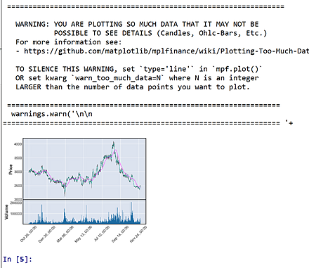
【関連項目】 Pandas, Python, Stooq, オープンデータ
教師あり学習 (supervised learning)
教師データ
教師データは,次の2つのセット.
- ニューラルネットワークの入力データ
- 正解データ
「訓練データ」などともいう.
教師なし学習 (unsupervised learning)
正解となるラベルのないデータを用いて学習を行うこと.クラスタリングなどがある.
距離学習
距離学習は,同一クラスであれば距離が小さく, 違うクラスであれば距離が遠くなるような数値ベクトル(数値の並び)を,機械学習によって得ることである.
距離学習は,2つの顔画像が同一人物であるかを判定したり,顔画像が既知の人物の誰であるかを特定したり(あるいは,既知の人物ではないと判定したり)する場合に役立つ.
距離学習と分類は違う.分類は,全クラスに属するデータを事前に得て学習させることを行う. 距離学習は,全クラスに属するデータを事前に得ることができないことを前提とする. 距離学習は,推論のときに,未知のクラスのデータが与えられる可能性があるなど,クラス数が不定である場合に有用である.
訓練
検証 (validation)
学習のときに,機械学習のモデルの品質を,検証用のデータを用いて評価する. 検証用のデータは,教師データとは独立したものである必要がある.
検定
検定には次のようなものがある.検定のときに,度数分布(ヒストグラム)をあわせて作成しておくことは,良い手がかりになる.
- パラメトリック検定
母集団は正規分布である.母平均,母分散を考える場合もある.
t 検定 (t test),F 検定 (F test), シャピロ・ウィルク検定 (Shapiro Wilk test), one-way ANOVA (One-way analysis of variance), ウエルチの方法による一元配置分散分析 (One-way analysis of means)
- ノンパラメトリック検定
母集団は正規分布とは限らない.
ウィルコクソンの符号順位検定 (Wilcoxon signed-rank test), マン・ホイットニーの U 検定 (Mann-Whitney U test, Wilcoxon rank sum test), コルモゴロフ–スミルノフ検定 (Kolmogorov-Smirnov test), クラスカル・ウォリス検定 (Kruskal-Wallis rank sum test)
交差エントロピー
多クラスの交差エントロピーは,
- yi : ニューラルネットワークの出力(yi の総和は1であること.例えば,ソフトマックス関数の場合は,総和は1になる).
- ti : 正解の出力.one-hot エンコーディングのクラス番号になっている.
のとき,次の通り.
-sigma_i( t[i] * log( y[i] ) )
2クラスの交差エントロピーは,
- yi : ニューラルネットワークの出力.{0, 1} の2値ベクトルになっていること.
- ti : 正解の出力.{0, 1} の2値ベクトルになっていること.
のとき,次の通り.
-sigma_i( t[i] * log( y[i] ) + (1 - t[i]) * log(1 - y[i]) )
勾配 (gradient)
勾配は,すべての自由変数について偏微分を行った結果として得られる ベクトルである.
機械学習では,モデル関数の偏微分を行った結果として得られるベクトルである. 重みに関する損失関数の勾配は,損失関数の値を最も減らすような重みの方向ベクトルである.
勾配消失問題 (vanishing gradient problem)
ニューラルネットワークの入力層に近い隠れ層について,その勾配が 0 に近くなる傾向のこと. 勾配が 0 に近くなると,学習における重みの変化が小さくなり,学習がうまく行えなくなる. LSTM (Long Short-Term Memory) は勾配消失問題を解決できるとされている.
混同行列 (confusion matrix)
分類モデル (classification model) での分類結果について集計した N かける N の表. N はクラス数である. 分類モデルでの分類として得られたクラスと, 実際のクラス(正解のクラス)とを,縦方向と横方向にする.
勾配降下法 (gradient descent)
モデルのパラメータについて,損失の 勾配を算出することにより, 損失を最小化する方法の1つ. 損失を最小化するような重みとバイアスの最適な組み合わせに徐々に近づけるために,パラメータの調整を繰り返す.
時系列データ (time series data)
時系列データは,「昨日の気温は15度,今日の気温が13度」のように,時間とともに,値が変化するようなデータである.
【関連項目】 Johns Hopkins 大の COVID-19 データレポジトリ
時系列データのニューラルネットワークでの扱い
時系列データをニューラルネットワークで扱うとき, 前回の推論時でのニューロンの出力の一部を,次の推論に反映させることが役立つ. 例えば,10月23日のデータでの推論時での ニューロンの出力の一部を,10月24日のデータでの推論に反映させるようなことである.
前回の推論時での出力の一部を,次の推論に反映させるために, 前回の推論時でのニューロンの出力が, 次の推論時で,同じニューロンの入力の一部になるようにするなどで,ニューラルネットワークを作る場合がある. そのようなニューラルネットワークには, リカレントニューラルネットワークがある. リカレントニューラルネットワークには, LSTM (Long Short-Term Memory), GRU (Gated Recurrent Neural Networks) などのバリエーションがある.
【関連項目】 GRU (Gated Recurrent Neural Networks), LSTM (Long Short-Term Memory), リカレントニューラルネットワーク
次元削減 (dimension reduction)
特徴ベクトルの特定の属性を表現するのに用いられる次元の数を削減すること.
収束
収束は, 学習において, 学習を繰り返したのち, 学習を1回行うごとの training loss と validation loss の変化がとても少なくなっているか,そうでないかを判断する場合に関係する.
主成分分析 (principal component analysis)
次の Python プログラムは,Iris データセットの主成分分析を行い,第1主成分,第2主成分,Iris データセットの属性 species で散布図を表示する.
次の Python プログラム では Iris データセットの主成分分析の第1主成分,第2主成分を横軸と縦軸の値として散布図を書く. 'species' を使って色を付けるとともに,形を変える. 縦軸のラベル,横軸のラベル,凡例の表示も行う.
import numpy as np
import pandas as pd
from sklearn.datasets import load_iris
import sklearn.decomposition
%matplotlib inline
import matplotlib.pyplot as plt
import warnings
warnings.filterwarnings('ignore')   # Suppress Matplotlib warnings
import plotly.express as px
from IPython.display import display

iris = load_iris()
df = pd.DataFrame(iris.data, columns=iris.feature_names)
df['species'] = iris.target_names[iris.target]

pca = sklearn.decomposition.PCA(n_components=4)
r = pca.fit_transform(df.iloc[:,0:4].to_numpy())

fig = px.scatter(x=r[:,0], y=r[:,1], color=df['species'], symbol=df['species'], opacity=0.4,
                 labels={'x': '1', 'y': '2', 'color': 'species', 'symbol': 'species'})
fig.show()
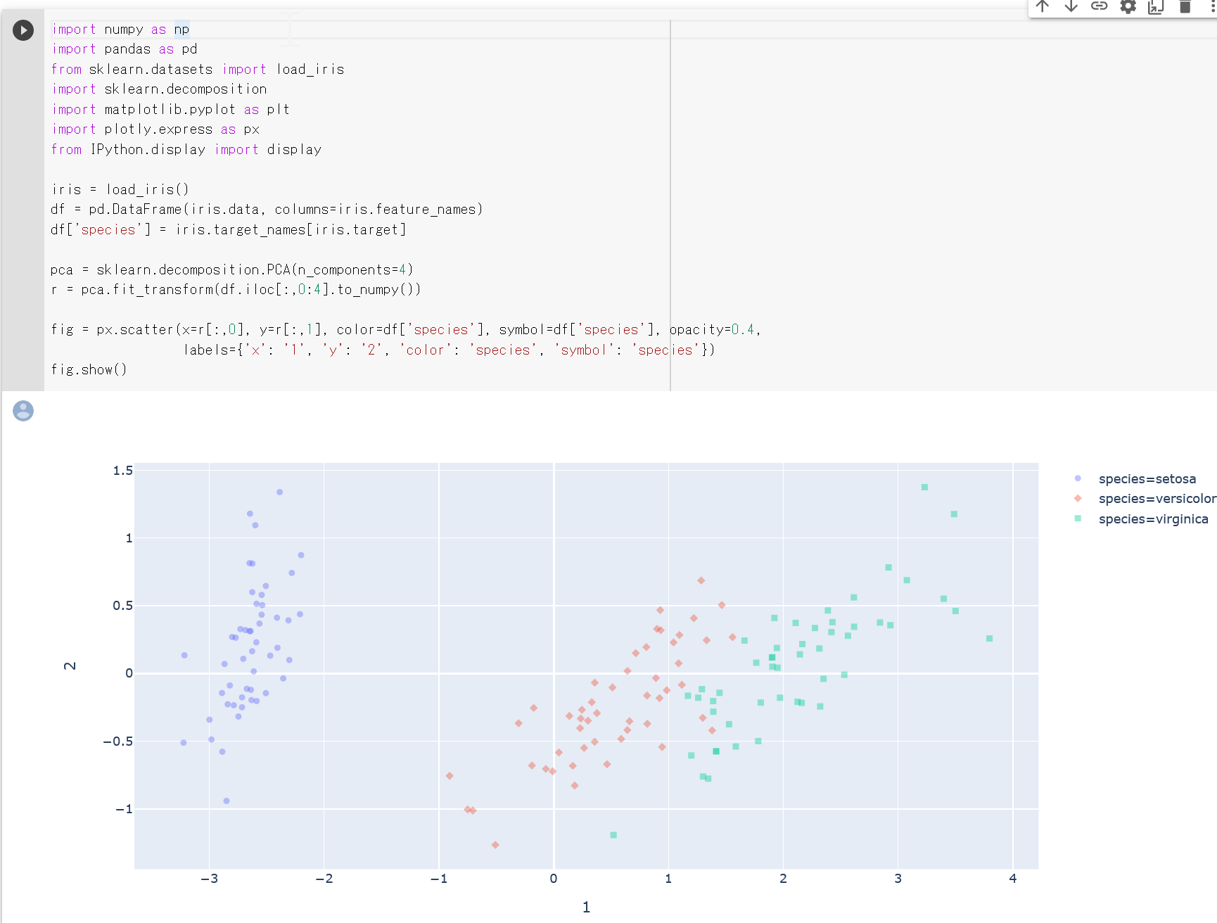
次の Python プログラムは,Iris データセットの主成分分析を行い,第1主成分,第2主成分,第3主成分,Iris データセットの属性 species で3次元の散布図を表示する.
次の Python プログラムでは,3次元の散布図のために, plotly の scatter_3d を用いている.
import numpy as np
import pandas as pd
from sklearn.datasets import load_iris
import sklearn.decomposition
%matplotlib inline
import matplotlib.pyplot as plt
import warnings
warnings.filterwarnings('ignore')   # Suppress Matplotlib warnings
import plotly.express as px
from IPython.display import display

iris = load_iris()
df = pd.DataFrame(iris.data, columns=iris.feature_names)
df['species'] = iris.target_names[iris.target]

pca = sklearn.decomposition.PCA(n_components=4)
r = pca.fit_transform(df.iloc[:,0:4].to_numpy())

fig = px.scatter_3d(x=r[:,0], y=r[:,1], z=r[:,2], color=df['species'], symbol=df['species'], opacity=0.4,
                 labels={'x': '1', 'y': '2', 'z': '3', 'color': 'species', 'symbol': 'species'})
fig.show()
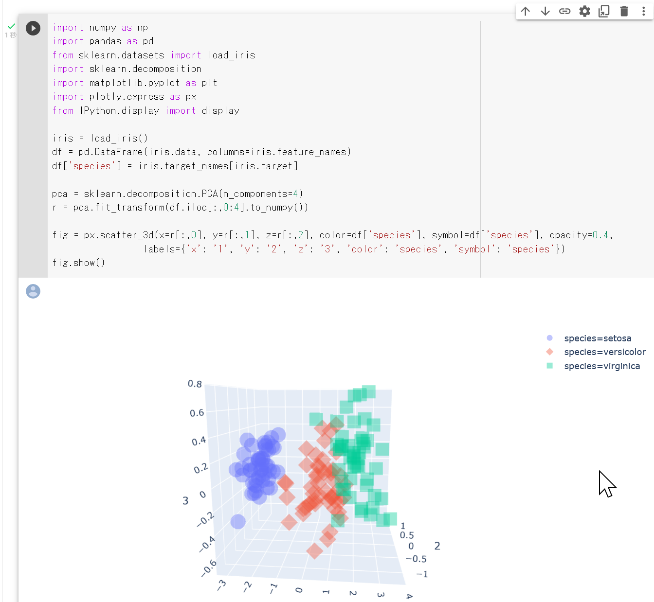
出力層 (output layer)
ニューラルネットワークの最終の層のこと.
正規化
正規化は, 値の範囲を,標準的な値の範囲に変換すること. 次のような意味がある.
- 複数のデータがあるとき,分布を保ちながら「データの範囲を0から1の間に収める」ようなデータ変換操作.
Python のプログラムは次の通り.
import numpy as np from sklearn.preprocessing import scale, minmax_scale minmax_scale(np.array([1, 3, 4, 5, 2])) - 複数のデータがあるとき,分布を保ちながら「平均 0,標準偏差1になる」ようなデータ変換操作.
Python のプログラムは次の通り.
import numpy as np from sklearn.preprocessing import scale, minmax_scale scale(np.array([1, 3, 4, 5, 2])) - 数値ベクトルがあるとき,そのベクトルの向きを保ちながら,長さを1にするようなデータ変換操作
Python のプログラムは次の通り.
import numpy as np
from sklearn.preprocessing import normalize
a = np.array([[1, 2, 0], [11, 12, 0]])
a.shape
normalize(a, axis=0)
normalize(a, axis=1)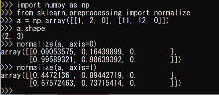
推論 (inference)
ニューラルネットワークを教師あり学習で使用する場合での推論は,学習済みのモデルに対して,入力を与え,出力を得ること. このとき,ニューラルネットワークの重みは変化しない.
ニューラルネットワークの重みが変化可能に設定したままの状態で推論を行うと,精度よく推論が出来ないなどの問題がある.PyTorch では,eval メソッドの実行により, ニューラルネットワークの重みが変化しないように設定した上で推論を行う.
出力は分類結果であったり,分類結果の確率分布であったり,さまざまありえる.
生成モデル (generative model)
生成モデルは,データ X とクラス C の結合確率をモデル化し, そのモデルのパラメータと,データ X の同時確率を最大化したもの.
あるいは,生成モデルのことを,データ X を生成するための確率モデルという意味でいうこともある.
正則化 (regularization)
正則化は,モデルの複雑さに対するペナルティととらえることができる. 正則化は過学習の防止,緩和に役立つとされる. 正則化には次のような種類がある.
参考文献: http://research.microsoft.com/en-us/um/people/jingdw/pubs/cvpr16-disturblabel.pdf
生成的 AI (generative AI)
生成的 AI (generative AI) は,大量のデータによる学習により,要求に応じた文章や画像や音声などを生成する能力を持った人工知能である.
【関連項目】 リカレントニューラルネットワーク
正則化率 (regularization rate)
重みと比べたときの,正則化関数の相対的な重要性を指定する数値である. 正則化率を上げると,過学習が減少するが,モデルの精度が低下する可能性がある. 正則化率を「lambda」と書くことが多い.
全結合 (Dense)
全結合は,多層パーセプトロン (MLP)で,ある層のニューロンすべてと,隣の層のニューロンすべてを結合すること.
全結合層
ニューラルネットワークの 層(レイヤ)のうち, 後続の層(レイヤ)と 全結合されている層(レイヤ)のことを 全結合層という.
「Fully-connected Layer」と言ったり,「Dense Layer」と言ったり,「Affine レイヤ」と言ったりもする.
層(レイヤ)
ニューラルネットワークは, 層(レイヤ)の積み重ねで構成されると考えることができる.
ニューラルネットワークの1つの層(レイヤ)は, コンピュータの中に作るとき,全結合層 (fully-connected layer), 活性化関数層 (activation layer) という複数の層(レイヤ)に分かれることが普通である. さらに Dropout のような,新しい層(レイヤ)が加わることもある.
入力の次元数が 784,ニューロン数 100,100,100の3層,クラス数 10,ドロップアウト 0.05 であるような分類モデルのプログラムは次のようになる.
m.add(Dense(units=100, input_dim=len(768[0])))
m.add(Activation('relu'))
m.add(Dropout('0.05'))
m.add(Dense(units=100))
m.add(Activation('relu'))
m.add(Dropout('0.05'))
m.add(Dense(units=100))
m.add(Activation('relu'))
m.add(Dropout('0.05'))
m.add(Dense(units=クラス数))
m.add(Activation('softmax'))
層構造のニューラルネットワーク
この資料で, 「層構造のニューラルネットワーク」というときは, ニューラルネットワークが層構造をなしていて,さらに,ある層(レイヤ)のニューロンは, 次の層(レイヤ)のみにつながる(つながりでは,飛び越しや後戻りがない)という場合のことをいう. Keras では,「Sequential」という.
例えば,次のような 10層からなる層構造のニューラルネットワークを考えることができる.
- 全結合層 (fully-connected layer)
- 活性化関数層 (activation layer) として ReLU
- 全結合層 (fully-connected layer)
- 活性化関数層 (activation layer) として ReLU
- 全結合層 (fully-connected layer)
- 活性化関数層 (activation layer) として ReLU
- 全結合層 (fully-connected layer)
- 活性化関数層 (activation layer) として Softmax
m.add(Dense(units=100, input_dim=len(768[0])))
m.add(Activation('relu'))
m.add(Dropout('0.05'))
m.add(Dense(units=100))
m.add(Activation('relu'))
m.add(Dropout('0.05'))
m.add(Dense(units=100))
m.add(Activation('relu'))
m.add(Dropout('0.05'))
m.add(Dense(units=クラス数))
m.add(Activation('softmax'))
相互情報量 (mutual information)
library(entropy)
X <- c(1,2,1,2,3,2,1)
Y <- c(4,5,5,4,6,5,4)
a <-discretize2d(X, Y, 3, 3)
mi.plugin(a)
chi2indep.plugin(a)
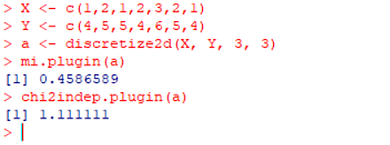
参考資料: https://cran.r-project.org/web/packages/entropy/entropy.pdf
相対度数分布 (relative frequency histogram)
度数分布のうち,データの個数を数え上げる普通の度数分布の他に, 比率(全体を 1 とする)を数え上げる相対度数分布 (relative frequency histogram), 累積値を数え上げる累積度数分布 (cumulative frequency histogram) がある.
scipy.stats.relfreq([0, 1, 1, 0, 0, 0, 1, 0, 0], numbins = 2)
参考ページ: https://docs.scipy.org/doc/scipy/reference/generated/scipy.stats.relfreq.html
library(entropy)
a = c(0, 1, 1, 0, 0, 0, 1, 0, 0)
discretize(a, numBins=2)/length(a)
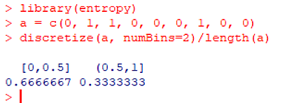
参考資料: https://cran.r-project.org/web/packages/entropy/entropy.pdf
損失 (loss)
ニューラルネットワークの出力と正解との差. つまり,損失は,モデルにより予測された値が,正解とどれだけ離れているかを示す. 損失の値を算出するために,損失関数が必要である.
損失関数
損失を算出するための関数のこと. 平均二乗誤差 (MSE, Mean Squared Error),カルバック-ライブラー情報量などがある. 「誤差関数」ともいうこともある.
ニューラルネットワークの学習においては,損失関数の値が最小になるように探索が行われる.
Keras の損失関数のページ: https://keras.io/api/losses/index.html
-
交差エントロピー (binary_crossentropy)
2クラスの 交差エントロピー (binary_crossentropy)を, 学習 (training)での,損失関数として使うことがある. logloss ともいう.
-
categorical crossentropy
多クラスの 交差エントロピーを, 学習 (training)での,損失関数として使うこと. マルチクラス logloss ともいう.
Keras の categorical crossentropy を使う場合には, ラベルのデータがバイナリ配列であり,その形状が (n_sample, nb_classes) であること. 2クラスの交差エントロピーを使いたいときは,binary_crossentropy を用いる.
大規模言語モデル (large language model)
大規模言語モデル は,自然言語処理を機械学習で行うためのモデルの一種であり,その中でも数億〜数十億以上のパラメーターを持ち,膨大な量の自然言語データによる訓練を受けたものを指す. 大規模言語モデルは,文章の生成,要約,翻訳,対話システムなどの自然言語処理において有用性が示されつつある. 代表的な大規模言語モデルには,OpenAI の GPT,Google の BERT,Meta の LLaMA,Stanford Alpaca などがある.
【関連項目】 FlexGen, LLaMA (Large Language Model Meta AI), LoRA, OPT, Stanford Alpaca, Whisper
多クラス
「多クラス」は,クラス数が3以上であること.クラス数が2の場合には「2クラス」という.
多クラスの分類 (multi-class classification)
2つ以上のクラスに分類すること. 2クラスに分類するときは binary classification という.
畳み込みニューラルネットワーク (CNN, Convolutional Neural Network)
畳み込みニューラルネットワーク (Convolutional Neural Network) は,畳み込み層 (convolutional layer) を含むような ニューラルネットワークである.
畳み込みニューラルネットワーク (Convolutional Neural Network) は, 次の3種類の層を含むように構成するのが普通である.
- 畳み込み層 (convolutional layer)
参考文献: Non-linear Convolution Filters for CNN-based Learning, CoRR, abs/1708.07038
- プーリング層 (pooling layer)
参考文献: A new kind of pooling layer for faster and sharper convergence, https://github.com/singlasahil14/sortpool2d
- 全結合層 (fully-connected layer)
【関連項目】 Applications of Deep Neural Networks, Keras, ディープラーニング
畳み込みニューラルネットワーク (Convolutional Neural Network) を作成する Python プログラム(Keras を使用)
例えば,次のような5層からなる層構造のニューラルネットワークの作成を行う.
- 2次元の畳み込み層 (convolutional layer)
- 2次元の畳み込み層 (convolutional layer)
- プーリング層 (pooling layer)
- 全結合層 (fully-connected layer).ニューロン数は 128.
- 全結合層 (fully-connected layer).ニューロン数は 10
その Python プログラムは次のようになる.
from __future__ import absolute_import, division, print_function, unicode_literals
import tensorflow as tf
from tensorflow.keras import layers
from tensorflow.keras import backend as K

gpu = tf.config.list_physical_devices(device_type = 'GPU')
if len(gpu) > 0:
    print("GPU:", gpu[0].name)
    tf.config.experimental.set_memory_growth(gpu[0], True)

# 畳み込みニューラルネットワークの作成
num_classes = 10
img_rows, img_cols = 28, 28
if K.image_data_format() == 'channels_first':
    input_shape = (1, img_rows, img_cols)
else:
    input_shape = (img_rows, img_cols, 1)

m = tf.keras.Sequential(
    [
        tf.keras.Input(shape=input_shape),
        layers.Conv2D(32, kernel_size=(3, 3), activation="relu"),
        layers.Conv2D(64, kernel_size=(3, 3), activation="relu"),
        layers.MaxPooling2D(pool_size=(2, 2)),
        layers.Dropout(0.25),
        layers.Flatten(),
        layers.Dense(128, activation='relu'),
        layers.Dropout(0.5),
        layers.Dense(num_classes, activation="softmax"),
    ]
)

m.compile(loss='categorical_crossentropy', optimizer='adam', metrics=['accuracy'])
print(m.summary())
補足説明は次の通りである.
- TensorFlow,Keras の機能を使用している.プログラム中の add,compile,Conv2D,MaxPooling2D,Dropout,Flatten,Dense は,TensorFlow,Keras の機能である.
- Keras では, 活性化関数層 (activation layer), ドロップアウト層 (dropout layer) も考慮する.
- 損失関数は categorical cross entropy に設定
- 最適化手法は ADAM を使用
多層パーセプトロン (MLP)
超解像 (super resolution)
超解像 (super resolution) は,低解像度のものを入力として受け取り, 高解像度のものを出力する. その結果,解像度が高まる.
- アルゴリズムによる方法 bicubic など
- 人工知能による方法 Real-ESRGAN,ESRGAN,SRGAN など
下図の左は ESRGAN (RRDN GANS) 法の結果, 下図の右は bicubic 法の結果.
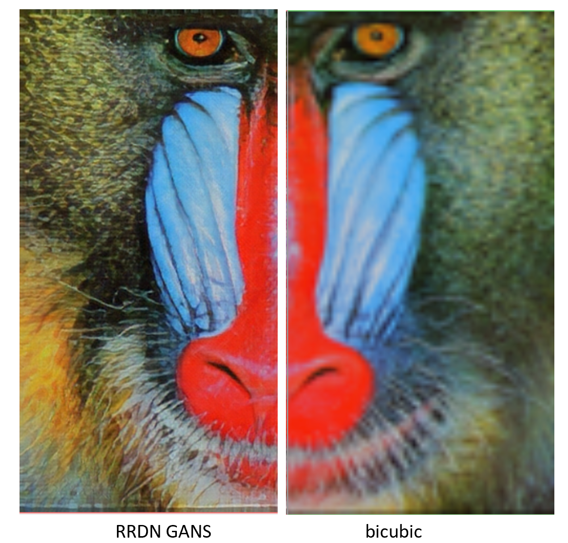
【関連項目】 Real-ESRGAN, ESRGAN
転移学習 (transfer learning)
ある機械学習のタスクから別のタスクに情報を転移すること.
ニューラルネットワークの転移学習では,学習済みモデル を使い,新しい分類を行う.新しい分類のための教師データを十分に準備できないときに効果を期待できる. 転移学習では, 学習済みモデルについて,重みを凍結(フリーズ)する. 学習済みモデルに新しい層(レイヤ)を追加して, 新しい分類を行えるようにする. 学習済みモデルは,新しい分類のための特徴抽出のために使うと考えることができる.
統計的機械学習 (Statistical Machine Learning)
統計的機械学習には,次のようなものがある.
- 変分オートエンコーダ (Variational Auto Encoder; VAE)
- 敵対的生成ネットワーク (GAN) など
特徴ベクトル (feature vector)
特徴値 (feature value) のベクトル.
度数分布(ヒストグラム)
度数分布のうち,データの個数を数え上げる普通の度数分布の他に, 比率(全体を 1 とする)を数え上げる相対度数分布 (relative frequency histogram), 累積値を数え上げる累積度数分布 (cumulative frequency histogram) がある.
library(entropy)
a = c(0, 1, 1, 0, 0, 0, 1, 0, 0)
discretize(a, numBins=2)
参考資料: https://cran.r-project.org/web/packages/entropy/entropy.pdf
Iris データセットの度数分布(ヒストグラム)をプロットする R のプログラム.
library(ggplot2)
p <- ggplot( iris[iris$Species=='setosa',]$Sepal.Length )
p + stat_bin(aes(hoge, ..count..))
凸最適化 (convex optimization)
凸最適化 (convex optimization) には, 凸関数 (convex function) での最小を発見する勾配降下法 (gradient descent) などがある.
入力層 (input layer)
ニューラルネットワークの最初の層.
入力の次元数
ニューロンの入力が数のベクトルであるとき,そのベクトルの次元数を「入力の次元数」という.
白色化
白色化 (whitening) とは,ニューラルネットワークの入力である数値ベクトルについて, 次のことを行う処理のこと.
- 平均が 0,標準偏差が 1 になるように変換する
- 数値ベクトルの成分の間の相関を除去する
微調整 (fine tuning)
2度めの最適化を実施することで, すでに学習済みモデルのパラメーターを, 新しい問題に適合するように調整すること.
「教師なしのニューラルネットワークで学習済みのものについて, 重みを調整することで,教師ありのニューラルネットワークとして使えるようにする」という意味もある.
転移学習では,モデル全体もしくはモデルの一部の凍結(フリーズ)を解除し,新しいデータで学習を行う.このとき,十分な量のデータを準備すること,そして,学習率を低く設定するなどで,モデルの改善を行う.
半教師あり学習 (semi-supervised learning)
教師データとして,正解の付いているデータと,正解の付いていないデータを使う. 正解の付いているデータを使い,ニューラルネットワークの学習を行う. そして,このニューラルネットワークに,正解の付いていないデータを与え,出力を得る. この出力を正解とみなして,正解の付いていないデータと合わせて,教師データとして使う.
深さ (depth)
深さ (depth) は,ニューラルネットワークの層(レイヤ) のうち, 重み (weight) についての学習を行う層(レイヤ)の数のこと.
物体検出
物体検出は,写真やビデオの中から,ある特定の種類の物体を検出すること.種類は複数ありえ,その場合には,物体検出が行われるとともに,その種類が判別される.
物体検出の結果は, バウンディングボックスで得られるのが普通である.
【関連項目】 ADE20K データセット, Box Annotation, COCO (Common Object in Context) データセット, DETR, Deformable DETR, EfficientDet, ImageNet データセット, Mask R-CNN, Max-Margin 物体検出 (Max-Margin Object Detection), MMDetection, MMPose, MMSegmentation3D, MMSelfSup, MMTracking, PANet (Path Aggregation Network), Pascal VOC (Pascal Visual Object Classes Challenge) データセット, RetinaNet, Seesaw Loss, SSD, YOLOv3, YOLOX, 顔検出 (face detection), セマンティック・セグメンテーション (semantic segmentation), インスタンス・セグメンテーション (instance segmentation)
分類 (classification)
分類は, データから,そのクラス名,もしくは,クラスについての確率分布を求めること. 「クラス分類」ともいう.
多くの場合には,ベクトルデータの集合を, オブジェクトをクラス(カテゴリ)に分けたり, クラスに属する確率を求める.
ディープラーニングによる分類は,事前に,教師データを用いて訓練(学習)を行う.
分類モデル (classification model)
Iris データセット を,3種類に分類する Keras プログラムの例は次の通り.
from __future__ import absolute_import, division, print_function, unicode_literals
import tensorflow as tf
import numpy as np
from sklearn.datasets import load_iris
import sklearn.model_selection
from sklearn.preprocessing import normalize
from IPython.display import display

iris = load_iris()
x = iris.data
y = iris.target

x_train, x_test, y_train, y_test = sklearn.model_selection.train_test_split(x.reshape(x.shape[0], -1), y, train_size=0.5)

NUM_CLASSES = 3

m = tf.keras.Sequential()
m.add(tf.keras.layers.Dense(units=64, input_dim=len(x_train[0]), activation='relu'))
m.add(tf.keras.layers.Dropout(0.5))
m.add(tf.keras.layers.Dense(units=NUM_CLASSES, activation='softmax'))

print(m.summary())

m.compile(
    optimizer=tf.keras.optimizers.Adam(learning_rate=0.001),
    loss='sparse_categorical_crossentropy',
    metrics=['sparse_categorical_crossentropy', 'accuracy']
)

EPOCHS = 300
history = m.fit(x_train, y_train, batch_size=32, epochs=EPOCHS, validation_data=(x_test, y_test))

# 分類
predictions = m.predict(x_test)
print(predictions.argmax(axis=1))
# 正解の表示
print(y_test)

import pandas as pd
h = pd.DataFrame(history.history)
h['epoch'] = history.epoch
print(h)

# 学習曲線
# https://www.tensorflow.org/tutorials/keras/overfit_and_underfit?hl=ja で公開されているプログラムを使用
%matplotlib inline
import matplotlib.pyplot as plt
import warnings
warnings.filterwarnings('ignore')   # Suppress Matplotlib warnings

def plot_history(histories, key='binary_crossentropy'):
  plt.figure(figsize=(16,10))

  for name, history in histories:
    val = plt.plot(history.epoch, history.history['val_'+key],
                   '--', label=name.title()+' Val')
    plt.plot(history.epoch, history.history[key], color=val[0].get_color(),
             label=name.title()+' Train')

  plt.xlabel('Epochs')
  plt.ylabel(key.replace('_',' ').title())
  plt.legend()

  plt.xlim([0,max(history.epoch)])


plot_history([('history', history)], key='sparse_categorical_crossentropy')
- 出力層のニューロン数は,クラス数と同じ one-hot エンコーディングのクラス番号を出力する
- 損失関数が categorical_crossentropy である
- 確率的勾配降下法 (SGD 法) を使う
- 確率的勾配降下法の学習率 (learning rate) は 0.01,Nesterov momentum を適用する.
- 「metrics=['accuracy'])」は accuracy を求めよという指示.
上のプログラムの実行結果は下の図の通り.
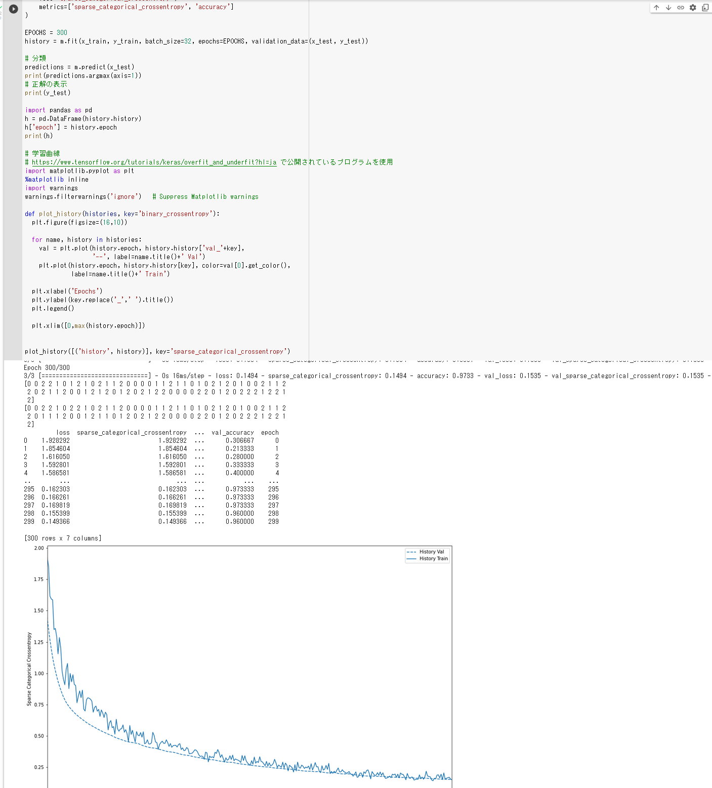
上のプログラムで作成される分類モデルは,次の通り.
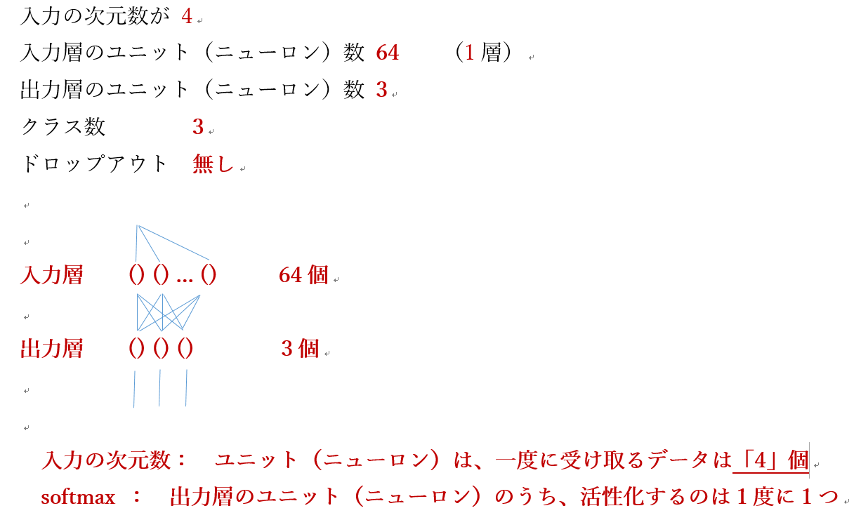
学習に追加に使うデータ: x_test と y_test のペア
- x_test:
全部で75行
入力の次元数は「4」なので,入力として一度に受け取るデータが4個(それを1行分).
- y_test:
正解データ. 全部で75行
print(x_train)
print(y_train)
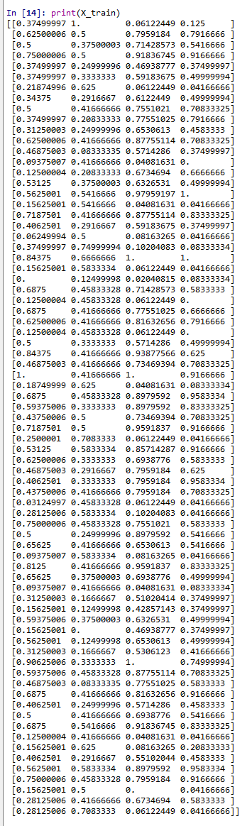
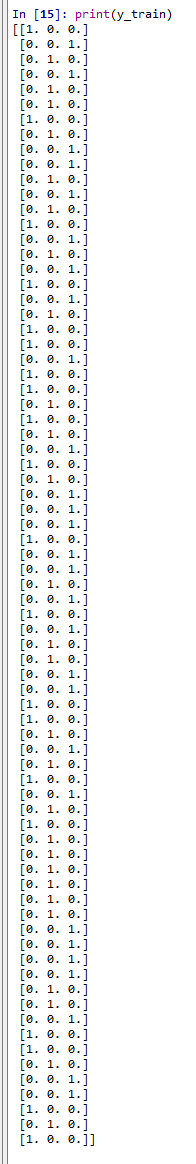
学習のあと,別のデータを使って分類してみる
まず分類したいデータの確認
print(x_test)
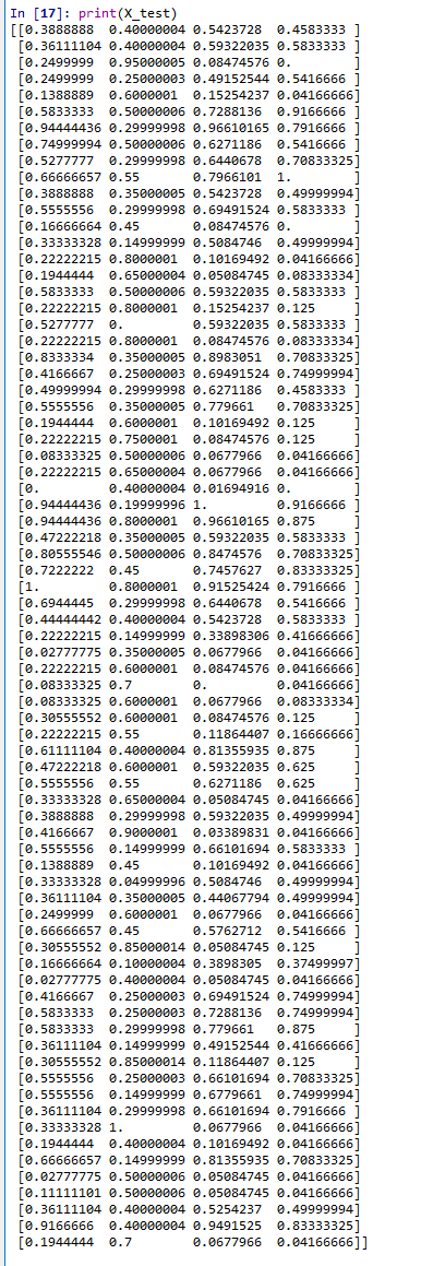
分類結果の確認
m.predict(x_test)
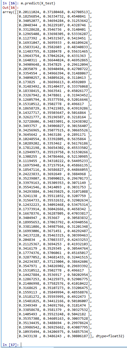
偏微分 (partial derivative)
変数が複数あるとき,ある特定の1変数を除くすべての変数を定数とみなした導関数のこと. 例えば,x に関する f(x, y) の偏微分では,y を定数に保ちながら微分を行う. x に対する f の偏導関数は,x がどのように変化するかのみに注目するもので,方程式内の x 以外のすべての変数を無視する.
変分オートエンコーダ (Variational Auto Encoder; VAE)
変分オートエンコーダ (Variational Auto Encoder; VAE) は,エンコーダとデコーダから構成される. 学習によって,エンコーダとデコーダのパラメータが決定されるもので,デコーダは,生成モデルになっている.
変分オートエンコーダ (Variational Auto Encoder; VAE) は,オートエンコーディング変分ベイズアルゴリズム (Auto-Encoding VB algorithm; AEVB algorithm) を用いた学習を行う. オートエンコーディング変分ベイズアルゴリズムは, 確率的勾配降下法を用いて,確率的勾配変分ベイズ推定量 (Stochastic Gradient Variational Bayes estimator) を極大化するような,エンコーダとデコーダのパラメータを求める.
その構造は,オートエンコーダに類似するが, 次の違いがある.
- オートエンコーダでの推論 (inference)は,入力と同じ出力を得ること.
- 変分オートエンコーダ (Variational Auto Encoder; VAE) での推論は,潜在変数の分布(ふつうは,単純な正規分布である)から,元データの分布を求めること.
変分オートエンコーダ (Variational Auto Encoder; VAE) は,CVAE と関連する.
- 文献
Diederik P. Kingma and Max Welling. Auto-encoding variational bayes. CoRR, abs/1312.6114, 2013.